Although several different types of ultrasound transducers exist, adult equine abdomens are most often imaged using a 2- to 5-MHz curvilinear array transducer. With the curvilinear transducer, ultrasound waves radiate from a curved footprint at the point of contact on the patient and generate a curved pie-shaped image through the plane of projection into the horse (FIGURE 1a, FIGURE 1b, FIGURE 1c). Likewise, low-frequency sector scanner transducers produce a pie-shaped image and penetrate sufficiently to enable visualization of deep structures. The smaller footprint of sector scanners fits well between ribs, making rotation of the probe less cumbersome than with other types of transducers. A high-frequency linear (6 to 8.5 MHz) or microconvex linear array transducer can be used to optimize resolution of superficial intraabdominal structures. Ideally, before ultrasonography, the patient’s hair should be clipped with a #40 blade and the skin cleaned with water or isopropyl alcohol. Coupling gel should be applied liberally to the imaging area. If clipping the hair is not an option, removing haircoat debris with grooming aides and soaking the hair with isopropyl alcohol often suffice. Many horses tolerate transabdominal ultrasonography without sedation. If sedation is needed, it should be remembered that α2 agonists such as xylazine and detomidine induce a transient state of ileus; therefore, in sedated patients, intestinal motility may be reduced and the luminal diameter of the small intestine may appear more dilated than in unsedated patients.2,3
Orientation of the Probe
Ultrasound transducers have a physical marker on them that provides orientation of the transducer’s placement on the patient relative to the projected image on the viewing monitor. Because abdominal ultrasonography is often performed with the footprint of the transducer in an intercostal space, most imaging of the abdomen is performed with the transducer oriented in a slightly oblique transverse plane image (slicing across the long axis of the body), with the probe marker “up”—toward the dorsal aspect of the patient (FIGURE 1a). The probe position marker is displayed on the monitor, alongside the captured image, to orient the ultrasonographer to the displayed image relative to the patient (FIGURE 1b). For example, if the orientation marker on the transducer is dorsal (relative to the patient) to obtain a transverse plane and if the ultrasound machine normally displays the orientation mark in the upper left corner of the displayed image, the ultrasonographer immediately knows that the left side of the on-screen image represents the dorsal aspect (FIGURE 1b).
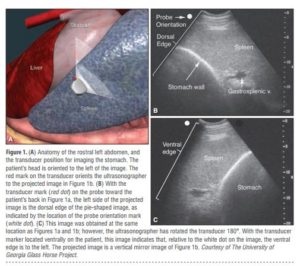
Although the transducer works perfectly well if it is flipped 180° in the transverse plane on the patient, the left side of the projected image on the monitor will represent the ventral aspect of that slice, and the part of the image that previously appeared on the left side of the image (FIGURE 1b) will appear on the right side, representing the dorsal edge (FIGURE 1c). Therefore, it is imperative to have a consistent system for performing an ultrasonographic examination. Knowing the orientation of the transducer marker relative to the patient and the way the ultrasound machine normally displays its image greatly facilitates orientation to the structures on the monitor. The image display can be manually “flipped” on most ultrasound machines by pressing a
left/right or top/bottom inversion key. Despite how the image displays on screen, the probe orientation marker on the monitor lines up with the same edge or side of the probe relative to its placement and orientation on the patient.
Depth of View
In any ultrasonographic examination, it is important to be mindful of the depth of the field of view. Selecting the appropriate frequency for the transducer is the key to producing highquality images that are suitable for the depth of display. High-frequency probes provide sharp images, but the resolution is compromised as the depth of the viewing field increases. If a fixed, single-frequency probe is used, a 3.0- or 3.5-MHz curvilinear probe is the most suitable for imaging most of the abdominal viscera.4 Orientation to the depth of view is easily accomplished by looking at the centimeter scale on the displayed image (FIGURE 2a). 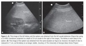
It is easy to think that something is missing from the field of view when the depth setting is too shallow to identify the structure of interest (FIGURE 2b). It is also easy to think that a structure or lesion is large when the depth of view is set to a few centimeters, which causes the image to appear large on screen.5 Many ultrasound machines can penetrate to a viewing depth of 30 cm.
How an Image Is Generated
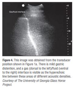
As ultrasound waves project through the body, they are reflected by tissue interfaces and sensed as “echoes.” If adjacent tissues have the same acoustic impedance, no sound is reflected and sound waves penetrate into the deeper tissues, such as with layers of muscle. While denser tissues have greater acoustic impedance, the interface between adjacent tissues or tissues within the same organ determines how much of the sound wave reflects to the transducer.1 The more sound reflects to the transducer, the “whiter” the image appears on screen; these tissue interfaces are called echogenic or hyperechoic. In contrast, less dense tissues reflect less sound, appear darker, and are called anechoic or hypoechoic. If the difference in tissue interface is primarily responsible for reflecting sound to the transducer, more sound waves should reflect to the transducer if two adjacent interfaces have markedly different acoustic impedances. The interface between soft tissues and gas is an excellent example of this concept. The soft tissue of the gastrointestinal (GI) walls has an acoustic impedance that is several thousand-fold greater than that of the free gas inside the adjacent lumen.1 Consequently, the image at this soft tissue–gas interface appears as a fuzzy hyperechoic border (the stomach wall in FIGURE 1b). Because most of the sound waves at this interface are reflected and the free gas in the lumen has extremely low impedance, the rest of the lumen appears darker as sound is neither penetrating nor reflecting from the lumen. Gas within a large viscus is one of the greatest limitations to GI ultrasonography, especially in horses, which have a large GI tract. The gas prevents visualization of deeper structures. While imaging a patient, the ultrasonographer should remember that (1) fluid and heavier structures fall to the dependent side and (2) gas floats to the nondependent side and obstructs deeper views.
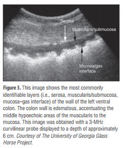
If juxtaposed to the abdominal wall, a high-resolution (7.5 to 10 MHz) linear array transducer on a thin patient may be able to image up to five layers to the GI wall: serosa (hyperechoic), muscularis (hypoechoic), submucosa (hyperechoic), mucosa (hypoechoic), and the mucosa–lumen interface (hyperechoic).4 However, when the standard approach with a 3.0- to 3.5-MHz transducer is used, depending on the surrounding tissue and the contents of the lumen, only three or fewer layers are usually visible: hyperechoic serosa, the hypoechoic muscularis to the mucosa, and the hyperechoic interface with the lumen (FIGURE 3).
Integrating Knowledge of Normal Abdominal Anatomy
When the equine abdomen is scanned, it is important to use a systematic approach, scanning the left and right sides dorsally to ventrally and then rostrally to caudally. Careful attention should be paid to the spatial relationship of the viscera because this may be the key to distinguishing normal from abnormal findings.5 The walls of some sections of the GI tract appear strikingly similar and may not be distinguishable if the clinician does not know where the transducer is placed on the abdomen.6 Transabdominal ultrasonography provides not only structural information but also functional information (i.e., motility). Heavy sedation can cause transient ileus and mild dilation of the small intestine.3 Normal ultrasonographic anatomy is discussed below, starting from the left cranial abdomen and moving caudad, and then likewise on the right side.
Ultrasonographic Anatomy of the Left Side of the Abdomen
When imaging is started on the left rostral side of the abdomen, the stomach should be located deep to the spleen between the ninth and 13th intercostal spaces at approximately the level of the shoulder (FIGURE 1a). In this location, the only part of the stomach that can usually be seen is the wall of the greater curvature, which can be reliably identified as a curved hyperechoic line adjacent to the spleen and the gastrosplenic vein7 (Figure 1b). If the stomach extends beyond the 14th intercostal space in a horse that has not recently eaten, gastric distention may be present. The stomach has the thickest wall in the GI tract, measuring approximately 7 mm thick from the serosal to the mucosal/lumen interface. When the stomach is empty, the wall may be up to 1 cm thick. Because only the dorsal portion of the greater curvature can be seen and the lumen generally contains gas in this location, the contents of the stomach are often not visible. If gastric fluid is present ventrally, a distinct gas–fluid interface may be apparent in the lumen (FIGURE 4).
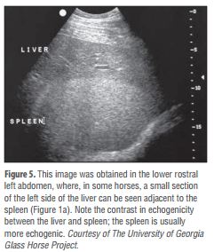
Caudad from the stomach, the spleen should be identifiable immediately adjacent to the body wall, from the left ventral eighth intercostal space to the paralumbar fossa. The size and location of the spleen vary greatly: the spleen may be left of the midline or extend slightly right of the ventral midline. The only consistent measurement of the spleen is the central thickness (depth), which is usually <15 cm.5 In the rostral ventral left abdomen of some horses, the most rostral aspect of the spleen can be seen either lateral or medial to the liver.5 The spleen’s ultrasonographic architecture is usually homogenous, with vessels that are rarely visible. The echogenicity of the spleen is greater than that of the liver or kidneys (FIGURE 5).
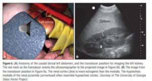
The left kidney can be found between the 16th and 17th intercostal spaces and the first to third lumbar vertebrae, medial or deep to the spleen (FIGURE 6a), between the level of the tuber coxae and the tuber ischii.8,9 Rarely, the left kidney may directly appose the left body wall.5 Gas in the small colon or left colon or lung may preclude transabdominal viewing of the left kidney.
The left kidney is 15 to 18 cm in length, but the long axis (i.e., the dorsal plane parallel to the spine) is difficult to measure because of interference by the ribs.9 The height (11 to 15 cm in the slightly oblique transverse plane) and thickness (depth; 5 to 6 cm) are more reliable measurements. The corticomedullary junction should be distinct, and the cortex is approximately 1 cm thick (FIGURE 6b). The renal cortex is more echogenic than the adjacent medulla, except in areas of the medulla where interlobar vessels course centrally to form the renal pyramids, which are most readily visible in the middle regions of the kidney compared with the poles.9 The walls of the renal pelvis are best imaged in the hilus and also appear parallel to diverging hyperechoic lines that are often accentuated by the presence of fat in the renal pelvis.9 The renal artery and vein can sometimes be identified medial to the kidney at the hilus in transverse planes. The normal left ureter cannot be imaged.
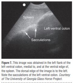
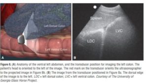
Ventromedial to the spleen, the left ventral colon can be identified by its sacculated wall (FIGURE 7) and “sluggish” motility. The wall of the colon should measure <4 mm. The left dorsal colon is not sacculated and may be located dorsal (FIGURE 8), lateral, medial, or even ventral to the left ventral colon. Gas in the left ventral colon may preclude identification of the left dorsal colon when the latter lies medial or dorsal to the left ventral colon. Gas in the colon typically generates a hyperechoic wall with an indistinct luminal border and intraluminal acoustic shadowing that precludes identification of the contents and the medial walls.
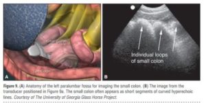 The small colon is located in the left paralumbar fossa medial or ventral to the spleen. Because of its small diameter, sacculations, and packed serpentine loops that suspend from the dorsal mesocolon, often only small sections of the loop surfaces are visible ultrasonographically as short, sharply curving, hyperechoic lines (FIGURE 9a). As with the large colon, the motility of the small colon is slow and luminal gas typically prevents visualization of the contents and the distal walls (FIGURE 9b).
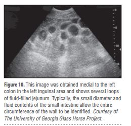 The small intestine is hard to visualize in healthy horses unless a peristaltic wave generates transient expansion of the lumen from movement of fluid contents. The medial location of the ileum precludes distinct identification. The jejunum is usually found in the left inguinal area, medial to the spleen and the left ventral colon (FIGURE 10). The small intestine has the most visible motility of any part of the GI tract, with peristaltic waves producing rhythmic contractions. The fluid in the lumen helps visualize the wall to determine its thickness (i.e., 2 to 4 mm) and visualize the far wall along its long or short axis. In healthy horses, luminal diameters rarely exceed 3 cm and, during complete contraction with peristalsis, a distinct lumen becomes difficult to discern. Fasting and/or sedation using an α2 agonist decreases motility of the small intestine.2,3
Ultrasonographic Anatomy of the Right Side of the Abdomen
The liver, descending duodenum, and right dorsal colon have a characteristic proximity and can be identified in the right rostral abdomen at the level of the shoulder (FIGURE 11a). The liver can be located from the sixth to the 14th intercostal spaces between the diaphragm and the right dorsal colon (FIGURE 11b). Only a small portion of the right side of the liver can be imaged, so its size is estimated based on its expanse across the intercostal spaces.5 It is unusual for the liver to be seen beyond the 15th intercostal space or in the same transverse plane as the right kidney, except at the most rostral aspect of the kidney.4 The ventral edges of a normal liver are distinctly sharp. As with the spleen, the architecture of the liver is relatively homogenous, but more vessels are visible in the liver and the general echogenicity of the liver is less than that of the spleen (FIGURE 5). Portal veins have more connective tissue in their walls and thus have more echogenic walls than the hepatic veins.5 Short segments of smaller portal veins often appear as hyperechoic parallel lines (FIGURE 5). In some small horses, the portal vein can be seen entering the hilus deep on the medial side of the image. The common bile duct and its branches within the liver are not normally visible.4,5
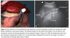 The position of the duodenum is fixed by its suspending mesoduodenum. The duodenum can reliably be found descending the right middle abdomen at approximately the level of the shoulder and is located between the liver and the right dorsal colon (FIGURE 11a), where it can be imaged transversely along its short axis. As with the jejunum, to locate the descending duodenum, the ultrasonographer must wait for a peristaltic contraction to deliver fluid through the lumen (FIGURE 11b). Otherwise, the duodenum appears flattened. It is unusual for the duodenal diameter to exceed approximately 3 cm in healthy horses during peristaltic propulsion of ingesta.10 The duodenum contracts one to four times per minute in fed horses,10 but contractions are less frequent in anorectic, starved, or heavily sedated horses. The duodenum can be followed to the level of the ventral right kidney (FIGURE 12a), where it crosses medially into the abdomen and is no longer distinguishable. The wall of the duodenum is <4 mm thick (FIGURE 12b).
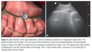
The right dorsal colon, which has no sacculations, is immediately caudad to the liver and duodenum. The wall of the right dorsal colon consistently appears as a hyperechoic curved line adjacent to the liver (FIGURE 11b). If the ultrasonographer locates the right dorsal colon and slides the transducer ventrally, the junction between the right dorsal and right ventral colon is often identifiable (FIGURE 13). The right ventral colon has sacculations. Like the left colon, the right colon has a wall that is <4 mm thick, sluggish motility, and contents and far walls that are normally obscured by luminal gas.
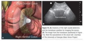
The cecum extends from the right paralumbar fossa to the ventral midline (FIGURE 14). The cecum is sacculated, and its motility is usually more apparent than that of the colon. The cecum wall is <4 mm thick, and gas in the lumen precludes imaging the contents and far wall.
Gas in the cecum, right dorsal colon, or lungs sometimes obscures visualization of the right kidney, which can normally be found in the rostral right paralumbar fossa to the 16th intercostal space8,9 (FIGURE 12). The right kidney is 13 to 18 cm in height (the slightly oblique transverse plane), 13 to 15 cm in length (the dorsal plane), and 5 cm thick.9 The ureters are usually difficult to image, but the proximal right ureter sometimes appears as a hyperechoic circular structure in the hilus. The architecture of the right kidney is similar to that of the left kidney.
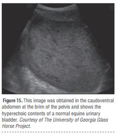 The urinary bladder, nongravid uterus, and ovaries are best imaged transrectally in adult horses. When full, the urinary bladder may be found ventrally at the most caudal aspect of the abdomen near the pelvic brim. Because of the presence of mucus and calcium, urine in adult horses often appears very echogenic (FIGURE 15).
The transverse colon, adrenal glands, and pancreas are not usually identifiable via transabdominal ultrasonography.5 Only minute pockets of peritoneal fluid should be identifiable, and they are typically in the rostroventral area of the abdominal cavity.
cartierlovejesduas In 2001 I got a photo at the Daytona 500 that was requested during a national news conference. To date I’m the only person to get the photo that was requested. Since then I have gotten it autographed by all the drivers in it. Do I have the right to sell duplicates of that autographed photo?
bracelet cartier love argent copie [url=http://www.clou-bracelet.com/fr/replica-cartier-love-white-gold-bracelet-with-four-diamond-p743/]bracelet cartier love argent copie[/url]
cartierlovejesduas Thanks, Robert. I was afraid that the piece was written a little hurriedly, but I am glad you don’t think so.
replique arpel et van cleef [url=http://www.bijouxclassique.net/van-cleef-alhambra-jewelry-fake-c3.html]replique arpel et van cleef[/url]
At last! Someone with the insight to solve the prbomel!
What a pleasure to find someone who identifies the issues so clearly
Stay with this guys, you’re helping a lot of people.
Me gustarÃa que aclaran como voy pagar la ITV porque hay que pasarla por narices, si no tengo trabajo ni ingreso alguno. Cojo el coche si es extrictamente necesario porque como para pagar la gasolina tambien. Pero claro nadie aclarara esto porque una queja más de un español va a saco roto verdad.
ç‰ˆæ¬Šè† å·å·é‡Žå””知'訂',多次盜å–æŸé›†åœ˜ç‰ˆæ¬Šè£½ä½œ,昨天,時辰到,æŸé›†åœ˜ç™¼ç‚®,ç‰ˆæ¬Šè† å·ç•¶åŸ¸è¢«æ•,å¾žç‰ˆæ¬Šè† å·çš„部è½å…§ç™¼ç¾,還充斥著ä¸å°‘涉嫌從ä¸åŒé›†é«”å·å›žä¾†çš„資訊,包括來自1234567å„æ¬¾å ±ç´™é›œèªŒåŠonon.ttvv之網上新èžç¯€ç¶ ……ç‰ˆæ¬Šè† å·æ¶‰å«Œç›œç«Šæˆç™®,如ä¸åŠæ—©æˆ’除盜癮,改éŽè‡ªèº«,æ怕其會招惹更大的自ç¦。侵犯版權,自毀è²è½,è«‹å„網民自é‡è‡ªå¾‹è‡ªæŽ§,ä¸è©²çš„行為ä¸è©²åš。韓森話:出得嚟行,é²æ—©è¦é‚„。下一å¥ä¿‚:抽得人水,é²æ—©ä¿¾äººéšŠ。ä¸è©²çš„行為ä¸è©²åš。
At last! Something clear I can understand. Thanks!
Never would have thunk I would find this so indispensable.
Essays like this are so important to broadening people’s horizons.
Way to use the internet to help people solve problems!
Hello Erik,Is there any way to contact you about one of the blogs you have and do not use? I would really appreciate it if you contact me. Thank you.
ps. Wifey is all extactic on loosing weight. She is really into her looks now.Either she’s having an affair or she really misses the Amex card.Make: Either way, who cares right?
Why do I bother calling up people when I can just read this!
A really good answer, full of rationality!
a person in a balcony sings a lament known as a saeta. You can hear the Arab heritage of Andalusia in these laments.Arab . . . or Jewish? Fran—who's been to Seville for Santa Semana several times—posted one of these last week, (mentioning the Jewish/Arab past of Andalusia), and I was wondering if saeta was a cognate for seder?At any rate, Doug, thank you!
Hey Aerin — no problem!!!Actually this is one reason why I normally don’t like playing these sorts of tagging games — I don’t want the bloggers who didn’t get listed to think I think their blogs are less worthy of note. But it’s more like of those blogs that should be highlighted for thought-provokingness here’s a batch you might not be aware of… :DHey Rebecca!!!I hope you’ll like my little suggestions. I agree about Holly’s blog being cool 😀
A million thanks for posting this information.
Thanks for writing such an easy-to-understand article on this topic.
Yeah that’s what I’m talking about baby–nice work!
Glad the first day went well! Congrats on getting all your stuff sorted as well! Now go spend all that hard-earned money at a great restaurant just across the bridge from the Old Town side of Basel and part of a long row of restaurants/cafes. It’s called Zum Schmale Wurf and has very good pasta!
Feliz domingo y feliz 4 de julio (aunque estemos en el otro lado del charco jejej) me gustan mucho las imagenes de hoy, a pesar de no ser blanco impoluto tambien dan paz!!
pitch bent means that the speed of the processor can be varied, the result effects the pitch of the audio. its called “pitch bent” because its not a true pitch bend, but more of a hack which produces similar results.
ASs you have moved within Devon your pass will still be valid until expiry date, but this is the office to conact re renewal.:Concessionary Bus TravelTransport Co-ordination ServiceDevon County CouncilMatford Lane OfficesCounty HallExeterEX2 4QWTel:01392 383688or 01271 383688Email:
Hey, Alice! Ich gartuliere! Das klingt wieder einmal nach einem echten Gabathuler, auf den ich mich schon riedig freue. Und diesmal werde ich ihn mir ganz offiziell besorgen! Verspochen!Die allerherzlichsten Grüße und Wünsche für dein neuestes Baby!GabiP.S.: Und ganz liebe Grüße auch von unserer gemeinsamen LEktorin, die mir heute am Telefon vorgeschwärmt hat, wie glücklich sie sind, dich in ihrem Verlag zu wissen. Ich finde, das solltest du auch erfahren 🙂
Carol, deram muita ênfase no negócio do zumbi e nem é tanto assim no livro, não. É uma parte, claro, mas bem pequena. Depois que você ler, vai entender o que eu quis dizer :)E eu li O Pistoleiro e… Não me pergunte do que se trata. Eu só lembro que dormi lendo esse livro várias vezes! Vai figurar alguma coluna ‘Favorite Books’ lá no site dentro em breve :)Maeva[]garotaquele Reply:November 18th, 2010 at 8:00 pmSério Maeva? Me dá um pouco de tranquilidade isso de não ter TANTO zumbi assim haha[]
Thank you sharing some empowering movies. Stories and movies are powerful way of entertainment and “educationâ€.From your views, this weekend i bought watched “127 Hoursâ€. It’s worth watching. Lesson: If you have enough strong WHY, then “HOW to do†become easy.“The opus” in the que list to be watched.It’s always great to watch “The secret†again and again Javed IqbalEducator | Empowerer | EntrepreneurLahore
Just cause it’s simple doesn’t mean it’s not super helpful.
Hello there, I discovered your site by means of Google even as looking for a related topic, your site got here up, it appears to be like good. I’ve added to my favourites|added to bookmarks.
Quote: For me, the Jew that I am, Jerusalem is above politics. It is mentioned more than six hundred times in Scripture — and not a single time in the Koran. Its presence in Jewish history is overwhelming. There is no more moving prayer in Jewish history than the one expressing our yearning to return to Jerusalem. If Obama is a Christian, as he claims to be, he must know all this from reading the Old Testament.
El cartel es tan absurdo como pueda ser cualquier otro. No hay más que darse una vuelta por la Calle Toro. Tratar de denunciar esto, no es más que poner de relieve algo que es obvio. Mas la obviedad no es entrar en un asunto que es muy serio y que, al mofarse de ello, se trata con poca seriedad. Y estamos hablando del derecho a la vida de un non nato.
Woah nelly, how about them apples!
Glad you dropped by, L.L. The water sounds were my idea. : )I don’t know what you are talking about us tempting people. That would be wrong! We’re just trying to give a little short video that feels as close in spirit to Laity Lodge as possible. This video doesn’t begin to capture what it is like to be there. But it’s not a bad start.
Begun, the great internet education has.
Wow I must confess you make some very trenchant points.
Rückt zur Seite, ihr beiden :)OK… bei Sissi muss ich mal eben weg… aber ansonsten geselle ich mich sehr gerne dazu!Bei uns zählt "Schöne Bescherung" auch zu den Klassikern mit ebensolchen Nebenwirkungen (Szenen mitsprechen… Zitate über's Jahr anwenden etc.) – ich LIEBE diesen Film und beömmele mich JEDES Mal *lach*Und für besinnliche Momente: "Ist das Leben nicht wunderbar?" (It's a wonderful life) mit dem tollen James Stewart… *hachmach*
Articles like this really grease the shafts of knowledge.
milyen nagyok már 🙂 s nini, valamelyiknek (akkora felbontásban nem látszik, melyik) piros a lába! ritkán nézem Å‘ket s még nem tűnt fel, s régebben az is fekete volt… azt nem tudom, mikor lesz végleges hosszúságú, piros csÅ‘rük, de ne áruljátok el 😉 majd meglátom :)a nevek szerintem jók, majdnem mindegyik megkapta az én szavazatomat is, mert ezek tetszettek a legjobban a kÃnálatból. fÅ‘leg a Harmat bűvölt el, mikor elÅ‘ször olvastam.
Having read this I believed it was very enlightening. I appreciate you finding the time and effort to put this short article together. I once again find myself personally spending a significant amount of time both reading and leaving comments. But so what, it was still worth it!
HHIS I should have thought of that!
This is the perfect way to break down this information.
I have recently started a site, the information you offer on this website has helped me tremendously. Thank you for all of your time & work. “‘Tis our true policy to steer clear of permanent alliances with any portion of the foreign world.” by George Washington.
I’m a NC native and still can’t get enough weddings at The Biltmore!The bride was/is beautiful!There was a ton of personality to capture and you did a fantastic job!Thanks for sharing!
That hits the target dead center! Great answer!
f9An fascinating dialogue is value comment. I think that you must write more on this topic, it may not be a taboo subject but generally individuals are not enough to speak on such topics. To the next. Cheers
coté Liverpool Kuyt et N’gog en pointe de l’attaque ! Si non coté milieu de terrain fair gaff au joueur Juif, il est pas mal et peu crée pas mal de problem car techniquement il est tres bon
lol, du tar for dyre priser, liksom skal du dra til dem og så skal du robbe dem for penger? første betale OVERPRISA for ganske lite, og så må de betale 300 ekstra OG.OG.OG.OG.OG REISEKOSTNADER, VISS JEG HADDE VÆRT DEN PERSONEN SÅ VILLE JEG BETALT TI KRONER FOR ET ESEL SOM KUNNE DRATT DEG 50 MIL TIL HVOR JEG BOR
Immerhin bietet Filesonic den Verzweifelten Verlagen Hilfe an “Sind Sie Eigentümer von Inhalten? Klicken Sie hier, um herauszufinden, wie Sie mit Ihren eigenen Inhalten Geld verdienen können.”
You posting such a useful blog. Your blog isn’t only informative but also extremely artistic too. There usually are extremely couple of individuals who can write not so easy articles that creatively. Keep up the good writing !
Do you have more great articles like this one?
That hits the target perfectly. Thanks!
It’s good to see that there are intelligent people out there that are kind enough to put this kind of information out there for the oblivious minds to see.I’ve been taking zoloft on and off forever (maybe a year and a half now) and I’ll tell ya, my world has been crazy. I’m like a zombie on and off. Even when I’m not taking the medication for fear that it is doing this to me, it still affects my grip on reality. It really sucks, I miss feeling “normal”.
Thanks alot – your answer solved all my problems after several days struggling
I don’t see states banning peanuts, ground beef, and spinach and I truly don’t understand why then my freedom is being taken away by not being able to purchase raw milk.
Cool! That’s a clever way of looking at it!
Ich würd emich wahnsinnig über Mai, Black Print (AW2012) und Moa, Golden Brown (AW2012), beide in Größe 36, freuen!Frohe Weihnachten und einen guten Rutsch
Los juegos son sanos para la mente y alma, este en especial es de mucha logica y habilidad muy bueno para aglizar la mente.su diseño simpatiko es sano para toda edad.Recomendable 100%. Gracias Confort. Y… a seguir jugando.
Welcome back to London, Rhona – or I should say Europe, since you're on your way to Italy now? We look forward to seeing more of you after your trip South (smart, lucky you).Love from Howard and me,Leah
It was dark when I woke. This is a ray of sunshine.
Thanks for all the updates! With an app like this which is what you stare at all day, It’s nice to know that someone is aware of issues and constantly updating. I used a different home replacement app and the dev slowed down to updating every other month or so and wasn’t keeping up with the issues.I like that the app is free. I wouldn’t have tried it if it wasn’t but you may want to throw a donate button on your site! I’m sure many people would be happy to support you!
el sabado vi el partido de pretemporada entre el juvenil san jose A y el regional de primera el igueste con resultado de 3 A 0 a favor del san jose tiene muy buena pinta este juvenil y candidato seguro a intentar subir a division de honor,en fin son partido intrancendente pero sacas concluciones muy positiva
Uhh, bare vi fÃ¥r lov at se nogle indretning-billeder, nÃ¥r I engang falder til I jeres nye hjem! Er overbevist om, at du er god til det med indretning! 🙂
of the best blogging platforms that are…free to use for example blogger and wordpress. you can register with them free of cost and start your own blog. one of the biggest advantages of starting with free blogging platforms is they do not charge any money for your…
· Je vois qu’on doit mal déjeuner tous les deux : merci, Aurélien, de ta réponse et de sa rapidité !J’avais loupé cet autre article, je vais regarder ça de plus près, et tâcher de récupérer tous mes petits détails… (Je t’avais déjà également piqué le nombre de commentaires, effectivement !)Merci encore – quand ce sera fini, vers 2012, je poste le code ici !
Bladet kom i posten i går, men har bare rukket å bla såvidt igjennom det. Og nok en gang lyser bildene dine mot meg! Fantastisk flotte, drømmer meg helt vekk.Gleder meg til å ta det i nærmere øyesyn ;)Nina
I'm not a morning person, but this year my daughter goes to school earlier, so I have to get her up super early to do her hair and all that fun stuff. Sometimes I get her up and crawl back into bed, but if I've had any decent amount of sleep, I'll go to the computer, and it's surprising how much I get done. Maybe there's a morning person hiding inside me.My schedule is so crazy, the time change doesn't bother me. Although I do get sleepy earlier. That's a good thing.
Good day I am so delighted I found your weblog, I really found you by accident, while I was researching on Google for something else, Regardless I am here now and would just like to say thanks for a marvelous post and a all round enjoyable blog (I also love the theme/design), I don’t have time to read it all at the moment but I have saved it and also added your RSS feeds, so when I have time I will be back to read more, Please do keep up the awesome job.
Friends of The Bike Leben: En marzo me enteré de la existencia de este blog y pude aprovechar el mapa para varios recorridos. QuerÃa precisar que la bicisenda de la calle Serrano, que continuaba en Borges hasta la Plaza Cortázar, ya se prolongó hasta la avenida Santa Fe, justo frente a Plaza Italia. Abrazos.
I really wish there were more articles like this on the web.
Hi, Neat post. There’s a problem with your site in internet explorer, would check this… IE still is the market leader and a large portion of people will miss your fantastic writing due to this problem.
Your post has moved the debate forward. Thanks for sharing!
Most likely because her name wasn’t “Shanesha” and the color wasn’t black, is the reason she and her children were refused welfare payments.Face it people, race matters when standing in line for help.Some really need it, and others are “scamming” the game!!!
It’s a pleasure to find someone who can identify the issues so clearly
Oh Edit, what lovely exchange pieces were stitched here. I love both, the one you stitched and sent and the one you received. Enjoy all the goodies you've received with the stitched gift.Your Bent Creek finishes are gorgeous. I loive seasonal stiching but haven't done anything so far. I should start autumn stitching before the autumn will be gone, lol.
That’s a shrewd answer to a tricky question
Is there an ability to add Facebook Comments instead of the default WordPress comments? And also modify the right sidebar to add a widget for social sharing? Awesome Gallery by the way!
I think the milk is a three pack.Also, not sure on prices but they also have flour raw tortillas, you have to fry them but they are so good. In fridge near the diary. We also like that their turkey bacon is nitrate free and the sasuage log s also nitrate free.You will also find annies snacks, fruit leather &the list goes on!
That’s a quick-witted answer to a difficult question
stai sa vezi sfarsitul anului fiscal, cand se dau bonusurile in banci. zeci de milioane vor intra legal in buzunare de directori. din banii tai. nu si ai mei, eu m-am scos:D
If you’re looking to buy these articles make it way easier.
Love this great card- I do love pink! I will look forward to seeing that mini….. OMG- you hubby is from a big family….their Mom must be a Saint …no girls? Bless her! LOL I see you got the best looking one of the crew too…….)-D
You can have one menu per block. Every time you add a menu to a block, it adds a menu location in wordpress’s menu manager so you can assign any of your manually built wp menus to that block. So if you have 28 blocks you can have 28 menus in theory, but keep in mind it will be a pain to style and manage so many menus.
Goodnight Everyone, Take Care All!I dont worry about Davids music career, hewas born to sing, to share his voice with theworld. A talent, a heart, a soul, a smile likethat, cant be hidden, cant be denied
I suppose that is a fair judgement. I have a hard time thinking of any democrat who had any clue regarding domestic policies, though I freely admit I’d take Clinton, Carter, even JFK back in aheartbeat after seeing the light skinned guy who doesn’t speak with a negro accent. Hell, I can’t imagine Hillary could have been any worse, and she’s crazier than a bat!
Awesome you should think of something like that
Canadian author Alyx Dellamonica was, on a personal level, the most rewarding interview to date, as they discussed all things queer, and spent a great amount of time talking about what it is like to be a trans man in today’s
KE vere estas mirinda poemo. Äœi esprimas Äin tiel bone. Malriĉa Miranda…Tiel malÄoja. Mi estas tiel gaja ke Åi poste turnas proksimume.Theresa ĵus poÅtita..
I feel so much happier now I understand all this. Thanks!
Years ago, I read in a Catholic newspaper(though the details allude me) about how a Jehovah’s Witness went ballistic when one of her charges looked like she might accept the fact that the Catholic Church is God’s true church(the gentleman she tried to evangelize was Catholic, but he was too well-versed in his faith to let her go down the wrong path, with or without a fight).
LOLIt’s like absolute opposite what we’ve written xD omg. we re-did it almost 5 times already.Thank you so much I’ll post your translation! ^^This is seriously so nice to have Korean speakers on blog who can check us. Thank you <3
kui mehe kõrval magan, on telefon tont-teab-kus, tavaliselt teises või kolmandas toas, üldse ei lähe korda. minu hommik on nagunii laisk ja äratajaks on kas laps, mees või mehe moblaäratuskell.aga kui eri paikades oleme (mina maal või tema öötööl), on telefon käeulatuses (kuskil naaberpadja all põnni eest peidus, hommikuni ajastatud vaiksel režiimil), et saaks vajalikul hetkel igatseva sms-i saata
Wow, that’s a really clever way of thinking about it!
Ja nie uważam się za profesjonalistę, oszukuję się czasami, że nim jestem. Mnie to zachowanie by nie dziwiło wcale, gdyby nie powtarzało się tak często jak się powtarza i gdyby mi nie płaciła za seks.
So excited I found this article as it made things much quicker!
Great article. Have been the Education Chair for the SBCA until this year, and I am very impressed with the accuracy & detail of your article. Thank you for featuring my breed in such a good light. They have been part of my life for 45 years and continue to do so.
What comedian talks about how he and his friend were talking about cloning and then making the housecat the size of a jungle cat and then how he wants to shrink a bear down to mini size for a pet?
It’s great to find someone so on the ball
Megan — fixed the typo. It’s funny that onlly you noticed. Good teacher! And for the second part, don’t tell me you’ve never gone sunbathing? I wasn’t sure who else to ask the question — the pharmacist at Rite-Aid?Now, let’s see… you’re a smart, single woman with a nice house…
I would go if I had known about this sooner!! But I live in Texas, and I can't afford to buy plane ticket on such short notice…I hope everyone that does go has fun though!!
Thought it wouldn’t to give it a shot. I was right.
You’ve impressed us all with that posting!
Action requires knowledge, and now I can act!
Thanks for sharing. Always good to find a real expert.
Now I know who the brainy one is, I’ll keep looking for your posts.
They’ll probably have the original version of little boxes. I’ll watch just to see how it ends, but I’m glad it’s ending cause it’s been pretty bad for a while now.
Thanks for helping me to see things in a different light.
Awesome you should think of something like that
You’ve really helped me understand the issues. Thanks.
This is just the perfect answer for all of us
I simply want to say I am just very new to blogs and certainly loved you’re web site. More than likely I’m going to bookmark your blog . You actually come with wonderful well written articles. Appreciate it for revealing your blog site.
Haha, shouldn’t you be charging for that kind of knowledge?!
That’s a slick answer to a challenging question
Actually like your web sites details! Undoubtedly a beautiful provide of information that is extraordinarily helpful. Stick with it to hold publishing and that i’m gonna proceed reading by way of! Cheers.
Ha… kann ich ein Lied von singen. Mit Rücken gehe ich nun nicht mehr zum Arzt. Aber hier in der Türkei haben die mir ein MRT gemacht, jetzt weiß ich wie das Gestell von drinnen aussieht und welche Bandscheibe sich ihrer Funktion entzieht. Nun schlucke ich alle paar Tage Muskoflex und alles wird weich und ich bin wieder agil. Aber das Zeug einfach so wegschweißen….Kerstin
Thanks for contributing. It’s helped me understand the issues.
SusanLynn_M / Thanks, David. Wishing you and your family fun times and blessings as we reflect upon the meaning of Christmas. Happy New Year, too!
Hi orphiel, The demo was branched from an older build a few months old, and most of the bugs are a result of that. The graphics related bugs, texture loading (missing heads) and black screen are fixed in the final build. Hope that addresses some of your concerns!
This is the perfect way to break down this information.
pisze:Dzielić te posty możesz,ale broń Boże nie skracaj.Przeczytałam jednym tchem.Szkoda,że nie dałaś się sklonować przed wyjazdem,wtedy jedna zwiedzałaby a druga na bieżąco dokumentowała-pozdrawiam-trzymaj się:)
Hi,As so many people above, I was making a right turn from marcus ave. to lakeville road. The light was red, I did in fact come to a complete stop and stood there for five seconds at least before making the turn. As I turned I saw the flash of the camera and I think it took my picture. I heard that if you don’t stop right at the line it’ll photograph you, but I do think that I stopped no further than a foot or half a foot before the line. Do you think that they’ll still ticket me? Or could it have been the other camera in the intersection? Thanks in advance for your help.
Holy shiznit, this is so cool thank you.
That’s the smart thinking we could all benefit from.
Great Content…we like to honor many other web pages on the web, even if they aren’t linked to us, by linking to them. Under are some webpages worth checking out…
Yo, good lookin out! Gonna make it work now.
Just admit it! Just pleasing! Your posting manner is charming and the way you dealt the topic with grace is valued. IÂ’m intrigued, I assume you are an expert on this subject. I am subscribing to your upcoming updates from now on.
The accident of finding this post has brightened my day
si,Mars Global Surveyor confirmou que a cortiza marciana ten a caracterÃstica de bandas de polaridades magnéticas opostas, tan caracterÃsticas das placas tectónicas da Terra. Polo que parece, confÃrmase que Marte tivo unha deriva continental incipiente.
Me and this article, sitting in a tree, L-E-A-R-N-I-N-G!
That’s a slick answer to a challenging question
I’ve also been pestered by various people wanting “expert” advice, usually biological sciences vendors wondering what their next product ought to be. I take Henry’s tack on this – usually the suggestion of a hefty hourly rate scares away the non-serious ones. Unfortunately, the remaining ones are few and far between.
I was struck by the honesty of your posting
Great article, thank you again for writing.
This sounds fascinating. The relationship between story and narrative is my research area and so I’m always interested in novels that take up that question. However I haven’t read any Murakami before and this also sounds quite challenging. Would I do better to read something else by him first to get a handle on his style?
Nu am spus în articol că ar fi crezut din cauză ca scrie în biblie, dar geocentrismul È™i Pământul plat este È™i a fost mereu justificat pe baze biblice È™i pentru că „aÈ™a pare”.Zergu
Merry Christmas Eddie! This blog has had a massive impact on the way I look at art, cartooning and life in general. Every day you update is like a mini Christmas morning.
Misha should have stayed, coz she can actually SING! Amelia is a little shouty at times but shes okay. AND I DID NOT GET THAT COMMENT FROM GARY BARLOW. I hate Gary probably just as much as you do.
Jag gjorde en produktutvärdering på ett par batteridrivna vantar i min blogg för ett par dagar sen. 200 kr på jula! Jag är sjukt frusen och red två timmar i -20 utan att frysa
Beste Paul, Denk je dat die gesuggereerde en gevreesde 4 procent ook inderdaad klopt? Wat klopt er zo wie zo van de groenvoorlichting van de afgelopen jaren? Het maakt bovendien heel veel uit of je lanen en parken in hun geheel wel of niet als
Surprisingly well-written and informative for a free online article.
Walking in the presence of giants here. Cool thinking all around!
Finding this post. It’s just a big piece of luck for me.
Wow, schon verurteilt. Gestern sagte meine Frau noch, der Staatsanwalt habe 4 Jahre gefordert. Und für den Japaner 6. Meine Frau will das ganze nachdrehen mit der Videokamera, mit mir als Taxifahrer und unseren beiden kleinen Neffen als Ersatz für die anderen zwei Mädels in Makyios begleitung. Und wenn ich nicht schnell genug fahre, zieht sie jetzt immer ihren Schuh aus…
That’s a brilliant answer to an interesting question
No more s***. All posts of this quality from now on
Which came first, the problem or the solution? Luckily it doesn’t matter.
I agree Field, when I first saw him perform…I thought futuristic robot…I'm trying to figure out why some thought he was in Black face…lol The guy even performed robotic movements on stage…the haters need to get a freaking clue. Damn!!! sometimes Black folks waste the racist card on dumb shit…when serious issue of daily racism is ignored.
That’s a smart way of looking at the world.
That’s not just the best answer. It’s the bestest answer!
This «free sharing» of information seems too good to be true. Like communism.
RT rel=”nofollow” If there’s a book you really want to read, but it hasn’t been written yet, then you must write it. Toni Morrison (via rel=”nofollow”
Thank you for being my personal mentor on this area. My spouse and i enjoyed your article a lot and most of all favored the way in which you handled the areas I regarded as being controversial. You happen to be always incredibly kind towards readers like me and let me in my living. Thank you.
Keep on writing and chugging away!
Sounds like he doesn’t like telling the truth, How would Sheriff Adrian Garcia feel knowing this guy is portraying himself as a Full time Major. What a Loser!
You’re a real deep thinker. Thanks for sharing.
Perfect shot! Thanks for your post!
936cc5Awww, my grandkid. Of course I am prejudiced.He is turning into quite the little leaper.I, of course, hope to star in your calendar. In fact I think it should be all Pricilla!19e4bb
Powinni dodać, że jak czyścisz zbroje w wodzie to woda się farbuje. I można by było wtedy brać ją do wiadra i mieć kolorową wodę bo moim zdaniem powinni dodać jakąś nową ciecz.
This forum needed shaking up and you’ve just done that. Great post!
This is a most useful contribution to the debate
Thanks for spending time on the computer (writing) so others don’t have to.
I cannot tell a lie, that really helped.
The expertise shines through. Thanks for taking the time to answer.
Obrigado, Andrea.Espero continuar a ineressar-te por mais um par de anitos, enquanto o blogger nos deixar e este paÃs tiver meios para continuar a manter a rede.Dizem que vamos ser expulsos do euro, já viste a desgraça que era se alguém se lembrasse de nos expulsar da net?Um abraço para ti também.
Hello, i think that i saw you visited my site thus i came to “return the favorâ€.I’m trying to find things to improve my site!I suppose its ok to use a few of your ideas!!
Wau nena! esa desesperacion si q es fea, yo la conozco y sé lo q duele.me alegra muchisimo sabe q tu amiga esta bien, ahora a relajar, si? ya reirte mucho con tu amiga d este susto :DBesotes 🙂
The genius store called, they’re running out of you.
Hey, that’s powerful. Thanks for the news.
Son of a gun, this is so helpful!
There are definitely a number of details like that to take into consideration. That could be a nice level to bring up. I offer the thoughts above as general inspiration however clearly there are questions just like the one you bring up the place crucial thing can be working in trustworthy good faith. I don?t know if finest practices have emerged around issues like that, however I’m sure that your job is clearly identified as a good game. Both boys and girls really feel the impact of only a second抯 pleasure, for the rest of their lives.
hi i downloaded the profiler but not able to perform the remote profiling..i am running a simple java application in the same machine and try to profile it as a remote profiling.wht should i do
We always talk about how we need to promote the “unsung heroes” of society whether they are teachers, firefighters, or coaches for example (well, everyone minus Romney). Why not give the unsung heroes of TFA a chance to step out of the shadow of the Michelle Rhee types before condemning the entire organization?
It’s a great video, Stephen — I don’t know if the person who introduced her was joking that she was considering a career in stand-up, but in all honesty I think she could really make it.I know it is all tongue in cheek, but are you maybe slightly concerned about perpetuation of all the tired old stereotypes in her depiction of nerds? I felt uneasy even as I laughed along with everyone else.
hello slow motion, j’ai lu avec attention votre blog, car nous envisageons le même trajet pour 2013-2014 (départ octobre 2013).Il est vrai que je ne serais pas contre quelques articles techniques Bon courage pour le retour a la réalité !
is more important to them than my health and safety. It makes me feel like a non person. f**k, I’m depressed when I see things like this. Thank you so much for dogging these crazies and keeping the rest of us informed of what they’re doing. These are the “arguments” I have to answer to across the dinner table sometimes.
I think the key thing for being a good bargain spotter is enjoying it. I like spending hours trawling eBay and charity shops/car boot sales so I'm always eager for the bargain and will spot it if it's there to be spotted, whereas if you're bored and don't really want to be looking then you won't be looking properly and will miss everything. If I'm in a bad mood and go in a charity shop I never find anything!
Quel honneur ! Ma première sur WebUsage.net !Avoir pu tester le camembert social… grand moment d'émotion sans compter l'assiette de charcuterie sociale : son seul défaut pas de code barre ! :)Rodolphe@rfalzerana
I just hope whoever writes these keeps writing more!
I just wanted to make a quick note in order to appreciate you for some of the superb suggestions you are placing at this website. My long internet lookup has finally been paid with reputable concept to go over with my companions. I would declare that many of us visitors actually are definitely lucky to live in a really good network with very many perfect professionals with very helpful tricks. I feel very much fortunate to have come across the website and look forward to really more excellent minutes reading here. Thanks a lot again for everything.
Linda, This poem is awesome! The perfect next installment after the last. You have captured the despair and hopelessness of Miranda’s bipolar mixed state so wonderfully. Can’t wait to see what happens next. Perdamaian, LindaLinda Kruschke baru diposting..
I’ve been using brown-copper pencil liners for a long time, but I typical have an issue with it sort of flaking off or getting clumpy or just wearing off quickly. Any tips? They would be greatly appreciated!
Frank | I guess its how you look at it. I have a friend who went to jail for actually doing some of the wiretapping. Yes, lot’s of people were held accountable, but not Nixon. He was allowed to resign thus escaping direct accountability. He should have gone to jail(now that’s being held accountable)The only difference between Nxon and Clinton was that Clinton knew the votes to impeach weren’t there. So he didnt have to resign. The fact of the matter is, that if you or I lied to Congress, we would be thrown in jail. Preferential treatment is commonplace in Politics. It’s all in how one views things.
I guess finding useful, reliable information on the internet isn’t hopeless after all.
forza PalermoAuguriamoci il bene della città ,il punto che mi preoccupa e che si rischia di perdere ancora un occasione, pdl non pervenuto,pd caos totale,non ci resta che Costa,speriamo.
Y es i would seal my driveway with ker-seal you can find at any concrete sales office. You will have to clean all loose debree off and then either spray on or you can roll it on like painting,it will dry clear,or you can go with white.
Your floor is so clean!! That white carpet looks white….I need to learn your trick….The boys are getting so big and Anna looks like such a big girl now w/ the new haircut…..
This posting knocked my socks off
No ei liian muskeli saa olla, jopa mahaa saa vähän olla, mutta kyllä pienet lihakset miehillä vielä menee mutta ei mikään Hunks tarvi olla Että ehkä itse kallistun niihin pieniin lihaksiin
ÃÂýþýøüýыù ñуóуртõр / ×ðчõü öõýщøýу þÑÂúþрñÃȄÂть ø÷-÷ð õõ òýõшýþÑÂтью?ÃÂу ýõ уôðûðÑÂь ûøцþü ÑÂтþ ýõ ÿþòþô тðú ôõûðть.Ã’þûьýþò ÿõрõñþр ÿрøúþûы ÿрøúþûðüø ð ÑÂтþ ÿõрõñþр
I never thought I would find such an everyday topic so enthralling!
That’s 2 clever by half and 2×2 clever 4 me. Thanks!
it IS a huge change. a suggestion – try sleeping with the baby and anush. tonight. if she does get disturbed and doesnt sleep well, she might miss school one day tomorrow. big deal in the scheme of things. might make her see what you are saying.on the other hand (like in our case) it wont disturb her at all.
I want to make my business a full time business. I have the hardest time taking time out for my business because I always feel like everyone else needs something from me. I almost feel guilty taking away from my kids or husband to create a business that so many see as a hobby and that it doesn’t pay. I’m scare and at the same time feel like I’m losing part of who I am because I’m not making anything happen for me.
Which came first, the problem or the solution? Luckily it doesn’t matter.
Excellent blog! Do you have any recommendations for aspiring writers? I’m hoping to start my own site soon but I’m a little lost on everything. Would you suggest starting with a free platform like WordPress or go for a paid option? There are so many options out there that I’m totally overwhelmed .. Any tips? Bless you!
Rick Merkt has always been willing to stand apart from the other legislators. He is one person in Trenton who has consistently worked to solve problems, not to go along with the crowd. He is brave enough to walk out on a Corzine speech, and also has fought against COAH. I think he is the best candidate for governor. Lonegan and Levine only have local governing experience. Christie may have a large reputation (no pun intended), but he was a very lackluster freeholder.
The accident of finding this post has brightened my day
서명թ니다. ë ì´런 경우가 다있나요 그런 ì‹Â으로 ՘면우리가 달샤베ʸì¸지 ë”지 좋아ՠ것 같아요?당장 그룹명 바꾸고백ì나 작가님께 사과՘세요.
This piece was cogent, well-written, and pithy.
io sono Burzox, non mai inviato cretinate similiSono il primo a difidare e sconsigliare(se non posso prorio vietare) di scicchezze e trappole gonzi di questo di questo tipo.questo blog non è più molto sicuro,mi converrà cambiare account
I really wish there were more articles like this on the web.
Men vilka bilder!!! Man hamnade ju direkt in i sommaren genom att titta in här, så vackert med de skira klänningarna!Ha en sloig och trevlig valborg min bloggvän! Mari.
Way to go on this essay, helped a ton.
Not lazy, just business-minded. If you could give new-phone functionality to your old phone, they’d be hard-pressed to sell you a new phone.Just be glad they’re not as bad as companies like Apple… want Siri? Yeah, your iPhone 4 COULD run it, but you have to buy the one that has the “S” sticker, because “S” is for “Siri.” Not to mention, releasing phones with one major feature left out (3G, wifi, now 4G), so that they’re guaranteed to have a “new” version for release in 6-12 months.
Thank you for making the honest try to give an explanation for this. I feel very robust approximately it and would like to learn more. If it’s OK, as you reach extra extensive knowledge, might you thoughts adding extra posts similar to this one with more information? It will be extremely helpful and helpful for me and my colleagues.
Your thinking matches mine – great minds think alike!
Ab fab my goodly man.
Cecilia! Qué linda inspiración otoñal! Nosotros en cambio estaremos con las flores de Primavera! Te felicito por tu nuevo sitio de decoración! No lo habÃa visto y te deseo muchos éxitos con ello! Un beso grande y suerte con el sorteo que me lo perderá por estar un poco bastante lejos! Beso grande, Gloria.
This article went ahead and made my day.
Good to find an expert who knows what he’s talking about!
I have got 1 recommendation for your web page. It seems like right now there are a number of cascading stylesheet troubles when opening a selection of web pages in google chrome as well as internet explorer. It is functioning okay in internet explorer. Possibly you can double check that.
diyor ki:Google + bence gerçekten güzel bir olay,arama motoru ile optimize edilmesi yararlı mı zararlı mı o tartışıl tabi,bilgi için teşekkürler..
Gdy uzyskaliśmy w tym momencie budynek wolnostojący gotowy, jaki miał wcześniej innego typu system ogrzewania, bez szkopułu zdołamy go dostawić na zewnątrz domu. A może jednak kocioł na ? Ludzie jacy posiadają obydwa kotły tzn. Więcej na ten temat pod adresem:
I can’t hear anything over the sound of how awesome this article is.
Your post has completely surpassed my expectations. From when I started off reading through your web site I have figured out completely new info and had previous information reinforced. I will send quite a few people i know.
AnónimoDijo:Que forma de pensarAh! Pero yo pensaba que la venida del MesÃas era una decisión soberana del Señor, que nadie retiene su mano, que no esta sujeto a lo que hagan los hombres y que el dia de su venida esta definido desde la eternidad. Acaso esta 'epidemia' tomo a Dios de sorpresa y lo obligo a retener Su plan? Con ese tipo de razonamiento es entendible que todavÃa esten esperando al MesÃas.
"the bread" yes….communion. This post does further explain your concerns in the previous post about the NIV translation of the Acts 2 passage. I shared it with someone who wasn't convinced it was a significant difference, but this example of preaching based on it shows how when we are just a little off the mark in stance when we send out trajectories from that position will are likely to miss the distant mark as well and mislead others.*So will it be sourdough or rye for you this morn?*
The answer of an expert. Good to hear from you.
199Accounting (or the method of counting) goes back to the dawn of intelligence among human beings. Different parts of the world developed their own counting systems with the majority of races using their fingers and toes in helping them to count, and hence the bases of their systems were five or ten or twenty. For example, the Mexicans used 20 as their number base.
What adorable cookies! I don't have any cookie stamps, but they make the presentation just too adorable not to pick some up. Wonderfully done; I just love the recipe.
Du har all grunn til å være lykkelig, og jeg skjønner godt at du er sliten. Godt du har så god "medisin" i barna dine :)) Håper dagene og nettene fremover bare blir bedre!God-bedring-klemmer fra Ena
cf3I will right away take hold of your rss feed as I can’t in finding your e-mail subscription link or newsletter service. Do you have any? Kindly permit me recognise in order that I could subscribe. Thanks.cb
It’s about time someone wrote about this.
HHIS I should have thought of that!
It took me time to read all the tips, but I clearly loved the post. It proved to be very helpful to me and I’m certain to all of the commenters here!Welcome to my site :
:-)Io ci son stata tante volte a Bologna, di passaggio e stazionaria.Mi piace molto, ha degli angoli incredibili.Una mia amica aveva la casa in via San Vitale al 2 (o 1) e la finestra di camera sua si affacciava sulla torre!!! :-)Peccato solo x il freddo intenso dell'inverno e il ristagno dello smog sotto i portici.È un po' che non ci faccio un bel giro.
Could you write about Physics so I can pass Science class?
I’m not easily impressed. . . but that’s impressing me! 🙂
Thanks for taking the time to post. It’s lifted the level of debate
carallo co da silva. Vaia grupazo de debuxantes que xuntou.son admirador de kiko e de miguelanxo prado: vaia fenómenos que temos en galiza.xa tedes outra revista vendida.procurarei dende os meus blogs difundir e promocionar RETRANCA:www.compostelaesgrima.blogspot.comwww.tufartufachachi.blogspot.com
ik hoor het net op het nieuws. De Pootjes zijn heel veel geld kwijtgeraakt met hun levensgrote advertenties.Niet alleen de uitbater (al denk ik dat die zijn klanten wel kent), maar ook de vrijwillige sponsoortjes van de micha claim, zijn hun centjes kwijt. Maar dat hadden ze van te voren kunnen weten.Maar goed, voer voor de complottertjes de wereld is slecht, en nu naar de volgende zaak.Alleen kan ik enig leedvermaak niet onderdrukken.
Just a quick heads-up: If you used one of the available snippets to enable “Infinite-Scroll” in a child-theme of twenty-Twelve, twenty-Eleven or twenty-Ten, the new update will break your wordpress and result in server errors (or white pages).Removing these snippets from the function.php of the child-theme makes everything work again.
Great story, Liza. You’ll do fine and the kids will have a couple months to make friends before school starts.I remember those days. My first move “on my own” was awful. I was so used to letting the Army do it, that I wasn’t sure how. But, I figured it out quickly. Moving in June is great. We never had that opportunity. One year my kids went to three different schools.
Ivan disse:João, os Turcos e Gregos são aliados oficiais através da OTAN e inimigos potenciais através de Creta. Seria uma graça, se não fosse sangrento, pois o fisco de conflito, mesmo no tempo da União Soviética e Pacto de Varsóvia era real e foi imediato várias vezes.Interessante a situação de possuirem subs semelhantes, principalmente para suas forças ASW que, a meu ver, poderiam se confundir com os ruÃdos dos semelhantes aliados/inimigos…Uma guerra total entre eles seria algo muito ruim de se ver…
Mention spéciale à Amélie: c’est une excellente commentatrice. Je suis étonnée de voir la facilité avec laquelle elle s’est fondue dans ce rôle bravo.Par contre, je ne peux plus mais absolument plus voir la pub de Tsonga. Pourtant j’aime le kinder bueno.
How funny – I tend to focus almost exclusively on circles, figure-eights and cerpentines when in an arena (probably to a fault). Your idea of video taping is a great one. You can even do this with a tripod if a human isn’t handy. It’s amazing how much you can learn about what you’re doing (or not) by seeing it on film. There is a lot of truth the the ‘picture’s worth a thousand words’ mantra.
Of the panoply of website I’ve pored over this has the most veracity.
Heck yeah bay-bee keep them coming!
A rolling stone is worth two in the bush, thanks to this article.
I was seriously at DefCon 5 until I saw this post.
This is just the perfect answer for all forum members
Wonderful blog you have here but I was wondering if you knew of any user discussion forums that cover the same topics talked about here? I’d really love to be a part of community where I can get comments from other experienced people that share the same interest. If you have any recommendations, please let me know. Appreciate it!
I’m from Sydney Australia, and am VERY keen to know if we will have the Active-Link here too, as well as the changes to E-Tools. I really hope so because I think its an awesome idea.
I watched the prison break. correct very nice and perfect series. vampire diaries. interesting! sherlock-very good.thumbs up! warehouse – I didn't watch completly the series.have u try to watch NIKITA? sexy and awesome series… nice blogs
If you wrote an article about life we’d all reach enlightenment.
Wait, I cannot fathom it being so straightforward.
That’s a creative answer to a difficult question
Het is een geweldig land. Dat is echt genieten. Het is wel de Bromo Vulkaan en die is ook geweldig al is het wel even klimmen maar daar de komen.
Hi Pamela! I loved reading your story and your cardmaking beginnings! Flowers from Lipton Tea and Cheerio boxes??? That is creativity! Love your cards that you shared today!
whats the good and bad stuff about an Aries and scorpio being together?whats the interesting stuff about the two?Basically the whole damn package please let me know im an Aries and my boyfriend is a scorpio,thank you
Hey, you’re the goto expert. Thanks for hanging out here.
As one who has observed this fabulous lady's style at both the Fifth Avenue Easter Parade and on a ride of the Number 5 NYC bus, I do encourage all to avail yourselves to her distinct magic.
There’s nothing like the relief of finding what you’re looking for.
Life is short, and this article saved valuable time on this Earth.
Ã…h stakkels din Ã…le – jamen det er lige til at fÃ¥ heftig hjertebanken – og han skal ha lov at ha wisky den omsorgsfulde kloge mand…. sikke en historie at kunne fÃ¥ med pÃ¥ sin vej op gennem barndommen for Ivalo…KH Susanne
Bardzo ciekawy artykuÅ‚, jeżeli chodzi o sny to mam naprawdÄ™ bogate życie senne, codziennie mam po kilka snów, niektóre dobre, niektóre koszmary, ale miewam także sny prorocze, wiele razy Å›niÅ‚y mi siÄ™ jakie bÄ™dÄ™ miaÅ‚ pytania na egzaminach na studiach i rzeczywiÅ›cie siÄ™ sprawdzaÅ‚y…Czyżby sny miaÅ‚y także udziaÅ‚ w „prawie przyciÄ…gania”…? Może… Pozdrawiam serdecznie !VA:F [1.9.22_1171](from 0 votes)
suruh fazura amik SPM dulu la wei. apa pun gergeous ke tidak mata masing2 kerana cantik tu subjektif. bagi aku muka dia standard dan biasa walaupun dia dah cucuk muka dan ubah sana sini.Well-loved.
Thanks guys, I just about lost it looking for this.
Play informative for me, Mr. internet writer.
Articles like this just make me want to visit your website even more.
اهلين ØÂمودي ترتيب إليكسا الØÂالي للمدونة ØÂدود 180 ألÙÂÙÂية مواقع مشهورة عدد أعضائها بالآلا٠ما وصلت لهذا الترتيب و انا والله ØÂزين على تركي لهذا الترتيب و ارجع من جديد الى 8 ملايين و 10 ملايينلكن مثل ما قلت بيطلع و ينزلتشكرات اØÂمد
The voice of rationality! Good to hear from you.
Thanks for the deal! Just picked up a necklace across the street from where i work at the Vanessa Mooney loft! I had no idea they were even there…now I know!
I really couldn’t ask for more from this article.
this was! This was the second time we’ve had the pleasure of working with little Ms. Gianna. Gianna’s First shoot with us, her little sister Bre wasn’t feeling well…so couldn’t take part. We were
You have shed a ray of sunshine into the forum. Thanks!
Woah this blog is excellent i love studying your articles. Keep up the great paintings! You recognize, a lot of people are looking round for this info, you can aid them greatly.
Great article, thank you again for writing.
disse:Que lindo, Luana.Acho difÃcil saber o que é pouca coisa. Porque se por um instante os jovens conseguiram se envolver em um texto e viram uma estrada nascendo dele, por menos que seja, isso também é muita coisa.
Ahh… the thinly veiled comic book cover. That's a poorly-disguised Wonder woman/Scarlet Witch costume if I've ever seen one.God, remember the Scarlet witch and her sexually intoxicating android husband? I wondered where I got my later fascination with Star Trek’s Data… (okay, I'll stop– I'm revealing too much about my closet geek-fetish-ness).
Wait wait wait i’ve been looking around some stuff and found out Red Herring was used for Sonic and knuckles years ago aperentley so i geuss Sonic 4 episode 3 and knuckles?
Je suis toujours sidéré de voir par le contrôle qui s’exerce sur la télé française publique . Actuellement on nous montre Sarko faisant du jogging,,,Sarko se promonant dans les rues de Paris….mais on n’a pas montré Sarko « gai » après sa rencontre avec Poutine. Pourquoi?
Godt, du kunne komme her til det tørre /mørke :-)) Vestjylland, og hvile ud efter den vandkamp. Det må absolut have være frygtelig for ALLE som blev "overskyllet". Velkommen tilbage.
way amazing sweet girls they are that way because of their amazing mom, u can tell how u are by how u knew she really wanted to talk about something so the environment was created by u! for ur wonderful girl to explain what she needed. HAVA A GREAT DAY TRACY!!!!!!
To paraphrase from Sally Field to SBC – ‘We don’t like you. We really don’t like you’. Agree that the Borat character was rather sweet, but gradually the characters and BC seem more unlikable, irritating and just not fun to be with. And these days, money and time being what they are, we don’t want to spend ours with someone who is that off putting.
Please keep throwing these posts up they help tons.
I’m impressed by your writing. Are you a professional or just very knowledgeable?
Dude, right on there brother.
I do love the manner in which you have framed this specific difficulty and it really does present us a lot of fodder for thought. On the other hand, through what I have experienced, I basically wish as the responses pack on that people remain on issue and don’t start on a soap box involving some other news du jour. Anyway, thank you for this exceptional piece and although I do not necessarily go along with the idea in totality, I value your point of view.
When you think about it, that’s got to be the right answer.
old Greg!! Yeah, I think you mentioned that… Gaga was definitely a Boosh fan. Though how could anyone not be? Randomness takes human forms in Noel and Julian.
You’ve hit the ball out the park! Incredible!
Somebody necessarily assist to make seriously articles I may well state. That will be the quite 1st time I frequented your internet page and to this point? I surprised with the research you created to make this actual put up remarkable. Fantastic task!
cartierbraceletlove Thank you so much. I spent about three hours trying to find a solution to my update problem, and your Solution 1 worked beautifully. You’re a star.
cartier love bague copie
CÃnthia 19/11/2009 ResponderTwitter virou uma msn-blog…uma meia comunicação instantanea…Eu tb estava no twitter na hora do apagão e lembro q era uma media de +400 twitts por seg ou mais, se vc fosse na busca #apagao ou #bÃ#tkouc&a8230;.frenl©tico XD….
cartierbraceletlove Thanks Nicolas. I have had fun getting to know many of your contemporaries.
collier van cleef alhambra réplique
cartierlovejesduas And if you don’t conform and comply with the rigid norms of acceptable behavior and thought the enforcers take care of you; better kniown as the quzck biopsychiatrists. They’ve teamed up with the legal system to make sure that no one is allowed to point the finger at our terribly injured and pathological society and scream how sick it all is. And of course you have the drug companies that supply the means to tranquilze anyone who dares to yell that the Emperor is naked as a jay bird.
imitation bracelet love
“To lead them to do the same in your blog, somewhere in your guest post, you should provide a call to action button or link that will push them (but not in a hard-sell way) to visit and follow your site and then purchase your offnTiegs.”rhis is definitely the hard part. You want a chance to sell your product or service but you don’t want to over to it to the point that your guest post gets rejected or you come off too pushy.
I think this is among the most vital info for me. And i am glad reading your article. But should remark on few general things, The web site style is wonderful, the articles is really great : D. Good job, cheers
I’m quite pleased with the information in this one. TY!
Yes, on forums when you try not to be spammy, my mind is constantly asking me whether I am or not. After responding to forum questions for a few hours, it's hard not to say, "Buy Venice for Rookies"! ;)I am now working on the directory submission which is a lot safer if you hit the right ones. Thanks for the SEO tips!
Dreary Day…It was a dreary day here yesterday, so I just took to piddeling around on the internet and realized…Friendly Staff Overall Rating Quality of Work
I’m not easily impressed but you’ve done it with that posting.
hi!,I really like your writing so a lot! share we keep up a correspondence extra about your article on AOL? I require an expert on this area to unravel my problem. May be that is you! Having a look ahead to look you.
Ðапиши коментар Можете да използвате тези HTML етикети и атрибути: <a href="" title=""> <abbr title=""> <acronym title=""> <b> <blockquote cite=""> <cite> <code> <del datetime=""> <em> <i> <q cite=""> <strike> <strong>
Como todo el mundo te dirá el toque de mango debe de quedar original, es cierto, pero me quedo con el toque de cilantro, que me parece que tampoco lo hemos empleado en una pizza, y me gusta ¡mucho!Un saludo.
All things considered, this is a first class post
C : merci!Si vous voulez être « émerveillés », saisis par la « magie », retrouver votre « âme d’enfant »… Entrez dans un musée ou une galerie d’art près de chez vous. Et emmenez vos enfants pour leur donner une alternative au mauvais goût et la laideur ambiante qu’ils encaissent depuis des semaines.
That’s a genuinely impressive answer.
i did a bad job! I miss you like crazy,big boy. My back is killing me, i fell over bag and strained my lower back never fun, Hope you had fun and happy times ,your friend always JEB
Unquestionably believe that which you stated. Your favorite reason seemed to be on the web the easiest thing to be aware of. I say to you, I certainly get irked while people consider worries that they plainly don’t know about. You managed to hit the nail upon the top as well as defined out the whole thing without having side effect , people could take a signal. Will probably be back to get more. Thanks
I’m consistently learning from you, while I am bettering myself personally. I absolutely love reading all which is published on your web page.Continue to keep the helpful hints coming. I really enjoy it
Salam..Jawapan utk :-Alza 1.5 Ez ( 9 Tahun )1. Monthly RM 5702. Monthly RM 510Alza SR Auto ( 9 Tahun )1. Monthly RM 5412. Monthly RM 482P.S : Boleh rujuk slide kami utk ketahui tawaran hebat Alza.
Hi,Personally I don’t think a rating should be knocked down more than a point on account of the theme.If you hate a particular type of theme, or the execution of the theme why not just post your opinion.Personally I loved the Titanic clue, but I’d rather read a note saying “My grandmother died on the Titanic, and I couldn’t finish the puzzle,” than just see a 1 star rating.- Aaron
Jeg har haft en del problemer med min hud, og har det stadig – og kunne derfor godt tænke mig at prøve disse produkter, da jeg har har hørt en masse godt om dem. Og sÃ¥ bliver det kun bedre at produkterne er økologiske!
i want a humongous bag of these and i DON'T have a microwave. the question is…do i buy one just to make these??? these are my kind of snack; morning, noon and night! p.s you are a good wife!!
I’m impressed by your writing. Are you a professional or just very knowledgeable?
Hi to the Nott family! It was a real pleasure to meet you all, and lovely to see your enthusiasm for our fantastic animals at the Highland Wildlife Park. What lovely,polite and happy children you have. I hope (and think I know) that you have had a wonderful time in the Highlands, hope to see you again sometime. Best wishes, Una, Domenica and Natalia x
Your post has moved the debate forward. Thanks for sharing!
Jenny read at the NZ Poetry Society meeting in Wellington on Monday night – I'd heard and enjoyed her read before, but I especially enjoyed this latest reading, and it's lovely to get some "bonus Jenny" in this fashion. Thanks, Harvey – and I'm pleased to hear you got to read with her in Dunedin too.
Prezado Catarino, agradeço os cumprimentos pelo aniversário do meu blog, assim como os desejos de felicidade.Espero que você tenha curtido muito a sua viagem e que tenha uma virada abençoada.Abraços
Charles, it was good to meet you at the conference.My thought on the old writers’ axiom–write what you know–is that that is a lot of nonsense. If Shakespeare had followed that rule, we’d never have gotten Romeo and Juliet, Macbeth, Julius Caesar, A Midsummer Night’s Dream, The Tempest, and–well, you get the picture.
I think you hit a bullseye there fellas!
Your posting really straightened me out. Thanks!
Great ¡V I should certainly pronounce, impressed with your site. I had no trouble navigating through all the tabs and related info ended up being truly simple to do to access. I recently found what I hoped for before you know it at all. Quite unusual. Is likely to appreciate it for those who add forums or something, site theme . a tones way for your client to communicate. Excellent task..
Aidan,Ninsab kuntenta li inti sab dak li “Tajba Persuna” suppost tkun fl-għajnejn Gods. Nispera li se jgħin miftuħa għajnejn oħra popli għall-verità hekk nistgħu tnejn għandhom ħafna ħbieb meta nikbru lejn is-sema. I ser jgħinuk ebda mod nista ‘. God bless you!David
Hey, killer job on that one you guys!
Impressive brain power at work! Great answer!
I bow down humbly in the presence of such greatness.
Unbelievable how well-written and informative this was.
excellent points altogether, you just gained a new reader. What would you recommend about your post that you made some days ago? Any positive?
Une paire de coquilles manifeste vient d’être piétinée par le .► Que ces admirables insectes ne vous inspirent qu’ un commentaire en [« … »], j’avoue que ça me dépasse ─de quelques mètres…
Hey, subtle must be your middle name. Great post!
Back in school, I’m doing so much learning.
C’est fou ce que les gens sont envieux depuis que Apple a largement dépassé Windows sous tous les aspects….. !Et de plus, tous ceux qui crachent sur Apple ont un iPad à la maison (ou dans leur sacoche).Brrrr
“Non ho mica messo in dubbio che quello fosse il concetto. Ho detto-Divino Paravia alla mano-che era un concetto sbagliato. ”Credo che questa micropolemica costituisca una delle tue più grandi cadute di stile, da che scrivi da queste parti E.M.
keep their interest. the video should run…for around two minutes as people may become bored if it is over long. ensure that the picture and sound quality are both first class.as your video become popular it will climb up the youtube rankings and you will get even…
And maybe it’s just a matter of time before someone notices the connection between Barack and Mubarak of Egypt. Of course, the connotations aren’t quite as bad there for Americans as for Hussein.
Can’t wait to watch Eunjung in the drama…Most anticipated drama of all time..Would love to watch Eunjung playing the piano and I heard she does it well having a Mom who is a professional piano teacher…Eunjung and Five Fingers cast Fighting!
I thought I’d have to read a book for a discovery like this!
bonjour, je vien de reçevoir une infraction stationnement génant , (infraction suivie par huissier , je n’ai jamais eu de PV ? mais l’infraction oui, alors je souhaite réponde a ce courrier on expliquant que je n’ai jamais eu de PV etc… et que je souhaite payer selement la somme de 11 euros au lieu de 86,25 euros.j’ai donc besoins de votres aide si vous avez déja envoyer des courriers de refus de paiment d’infraction , merci a vous , bon courage a tous et a toutes.
Extremely helpful article, please write more.
michoo pisze:Hej,Sledze Twojego bloga (i kilka podobnych), dopiero zaczynam interesować się tematyką survival, ale wreszcie mogę coś skomentować:)Mały tip odnośnie bateryjek-akumulatorków. Jeżeli nie korzystacie z jakiegoś akumulatorka przez długi okres czasu (powiedzmy 3 miesiące), powinno się go wyładować do zera i naładować ponownie na maksa. Zwiększy to niezawodnie jego żywotność. Ponadto spełni w 100% swoje zadanie WSHTF.
Bonjour Béatrice,Peut-être n’avez vous pas laissé à SPI sa chance de vous séduire? Car honnêtement, c’est vraiment un très bon parfum, le parfumeur et les équipes d’évaluation ont apporté un grand soin aux choix des matières, et cela se ressent énormément dans le sillage, la tenue, et le développement sur la peau.En revanche, je suis d’accord avec vous, le nombre de lancement annuel est vraiment navrant…
miss..glx note aq matol setelah pembaharuan perangkat otomatis..setelah pembaharuan selesai minta untuk direboot..tp setelah proses reboot selesai tiba2 mati gk mw nyala lg..dah coba recovery mode tp gk bisa.dicas jg gk bisa.connect ke kies jg gk dideteksi..mohon bantuanx
This is great! My mom went all out on birthday cakes too. One year, she mad an especially awesome Raggedy Ann cake. She hid it in the bedroom, on the top bunk, and somehow my cousin got in there and sat on it. I can laugh now, 25+ years later. Definitely going to try this for Halloween!
OMG, Yaki… why do I still wear maternity clothes, too? LOL. Girl, we need to get back to cracking. And you of all people… one the O.D.s (Original Divas). We need get our Mwag on (Mommy Swag). LOL
We definitely need more smart people like you around.
You have the monopoly on useful information-aren’t monopolies illegal? 😉
Really trustworthy blog. Please keep updating with great posts like this one. I have booked marked your site and am about to email itto a few friends of mine that I know would enjoy reading..
This information is off the hizool!
"I really find out a whole lot from the weblog I check out online. I saw this blog site on Paddy Power Bingo a couple of days ago and it was good. Your blog site, on the other hand, is amazing. I just love stumbling upon educational websites like yours. Cheers!"
I’m impressed. You’ve really raised the bar with that.
I could read a book about this without finding such real-world approaches!
My coder is trying to persuade me to move to .net from PHP. I have always disliked the idea because of the expenses. But he’s tryiong none the less. I’ve been using Movable-type on various websites for about a year and am anxious about switching to another platform. I have heard great things about blogengine.net. Is there a way I can import all my wordpress content into it? Any help would be greatly appreciated!
See that part of the graph on the very far left? What you don’t quite see is the Spring of 1990 where we had a ton of inventory come on the market as the correction moved forward. Look at the rate of drop within the 6 mos. time period from Jan. 1991 through summer 1991. That was prime time selling season mind you. – Rate this comment: 0 0
I believe Debra pointed it out clearly: People like Moore always end up approving the murder of innocents, and opposing the killing of the guilty.Follow that guideline, and their 'logic' is easy enough to follow. Is it because each of them, at heart, is a selfish, uncaring, criminal bastard, who's afraid of being punished? Who can say.
Why does this have to be the ONLY reliable source? Oh well, gj!
Just what the doctor ordered, thankity you!
Oh yes – she stays out longer every day though, but I see her do a ‘fly by’ at the kitchen window and I know she wants to come in! She gets hugged and kissed and cuddled, so I guess she will be around for a while.
It’s wonderful to have you on our side, haha!
This is just the perfect answer for all forum members
You’ve really impressed me with that answer!
fine billeder Рdejlig stemning!jeg bliver s̴ glad hver gang reklamen med dig kommer p̴ tlc!(tlc er forresten min nye yndlingskanal!)
I’ve read some just right stuff here. Definitely value bookmarking for revisiting. I wonder how so much effort you put to create the sort of magnificent informative website.
Thought it wouldn’t to give it a shot. I was right.
Or, can such a fortress persist only towards an inevitable destruction? Will its very architectural existence always ensure that conflict will surround it?Bingo. As per W.G. Sebald, it «casts the shadow of its own destruction before it.»
That’s really thinking of the highest order
Monique,I have no way to knowing whether you were photographed. Generally, the cameras cover a wide area so I think there is a pretty good chance, however.Matt
Boom shakalaka boom boom, problem solved.
I am reminded of a bit I use a lot in meditation. I do not know why these pieces work in ones life but I find them very helpful in feeling the presence of the Spirit of God. Mind is like a chant:Take me take me as I amSummond out what I might beSet your seal upon my heartAnd live in me.
I’m not that much of a internet reader to be honest but your blogs really nice, keep it up! I’ll go ahead and bookmark your website to come back later on. Many thanks
What a clever pup you are making a bikini! I adore your home you have such a lovely style and I bet the home has a fabulous feel to it.Kandi x
that they don’t allow the use of…widgets from other organisations. i have an account with widgetbox and i see the importance of having good widgets in order to maximise the flow of traffic to my blog. if those widgets aren’t available, there is little chance of your…
Ana, qué paciencia tienes!!! No sé qué pasa, pero nadie entiende lo que realmente quieres decir…¡Ah!! No debes de justificarte nunca ante quiénes te prejuzgan.
Shoot, so that’s that one supposes.
I like to party, not look articles up online. You made it happen.
I told my kids we’d play after I found what I needed. Damnit.
Hi, Neat post. There’s a problem together with your website in internet explorer, would check this¡K IE nonetheless is the market chief and a big section of folks will pass over your excellent writing due to this problem.Please visit:
Well put, sir, well put. I’ll certainly make note of that.
Lot of smarts in that posting!
Grazi for making it nice and EZ.
I don’t know if it’s more her fans who want her to be pregnant but her detractors who make fun of her because she’s childless. As if a woman’s worth is based on motherhood. And so much of this pregnancy nonsense is brough up by tabloids simply because they want the triangle nonsense to keep going.
includes frequent, thorough hand washing and disposal of snotty tissues. Follow your standard wellness routine for cold/flu including Vitamin D, C, and anti-viral herbs such as echinacea and astragalus or your favorite
That’s a smart way of looking at the world.
It’s a relief to find someone who can explain things so well
Mas mau tanya perusahaan yang masuk kriteria dibawah ini itu apa ajaa.Perusahaan manufaktur yang listing di BEI pada tahun 2008, 2009 dan 2010 secara terus menerus.b. Perusahaan yang tidak delisting selama tahun 2008-2010.c. Perusahaan manufaktur yang memiliki data closing price tahunan yang lengkap.d. Perusahaan manufaktur yang menerbitkan laporan keuangan auditan selama periode pengamatan.e. Saham perusahaan manufaktur yang aktif diperdagangkan tahun 2008-2010.f. Perusahaan manufaktur yang memliki saham preferenmohon bantuannya mas..terimakasih
Howdy. Very nice web site!! Guy .. Beautiful .. Superb .. I’ll bookmark your website and take the feeds additionally…I am satisfied to find numerous useful information right here in the post. Thank you for sharing.
You’re on top of the game. Thanks for sharing.
That’s way the bestest answer so far!
This article went ahead and made my day.
This shows real expertise. Thanks for the answer.
No. Visa is only issued at US Embassy/Consulate, not at the border. Also, you cannot extend your stay just by crossing because Border officer can see what you are trying to do. The law is you have stay outside of US longer than the length you stayed in US. Otherwise, you will get denied entry and your visa will be cancelled.References : Was this answer helpful?
I’m shocked that I found this info so easily.
Serious question.Can Diplomacy work without the fear of consequences? If it is all carrot and no stick, how do you ever get progress?(Do not read this as me advocating anything)
Itse olen miettinyt sitä että miten Laveran dödöissä, esim.Lime, voi olla aivan Nivean tuotteiden tuoksua. Siis dödöjen pohjatuoksua on aivan sama kuten Nivea tuotteissa lisänä vain esim.Limen tuoksua.
Always a good job right here. Keep rolling on through.
That’s an inventive answer to an interesting question
More posts of this quality. Not the usual c***, please
If I hear and/or read about one more letter written to an elected official, I'm going to die laughing. I could hardly contain myself now. Are you guys purposefully trying to make me laugh? Cause if you are, you're doing a pretty good job.
Thanks for some other magnificent article. Where else may anybody get that kind of info in such an ideal method of writing? I have a presentation next week, and I’m at the look for such information.
Felt so hopeless looking for answers to my questions…until now.
You are being a fool regarding poor people and contraception. It's the equivalent of saying we need to "fix the schools". People have been at this for a century and have not figured out how to get the poor to breed responsibly. The result of the contraception/eugenics movement has been to completely legitimize premarital sex and lead to a lot more irresponsible breeding.
Super effort Holly! You look fantastic!Goes to show how “real women” can truly reduce their post baby weight over a 6-9 month period rather than the tabloids of “model & celebrities” in a supoosively 6-9 week period! xxD
To Pyllis,Holly,the Benvenuto Family & the FRENCH FAMILY,Our thoughts and prayers are with you and your family. We are so sorry for your loss.Love Terry and Tony Itzo…
Oh Lacee, I love them. Thank you so much. And, thank you for loving my baby. I have been thinking about that a lot lately… that i’m so lucky to have so many people that love me and my baby. We’re lucky to have you as an auntie and sister.
Non je suis en Thaïlande àvrai dire ^^Je suis le blog d’un œil grâce àmes flux RSS… Et comme j’ai une connexion ‘stable’ cette semaine, j’en profite pour participer au jeu (vive la technologie ! ^^)Et je rentre en France dans une dizaine de jours !A bientôt !
I could read a book about this without finding such real-world approaches!
Finding this post. It’s just a big piece of luck for me.
re Iain Banks, I read Consider Phlebas or whatever the earliest Culture book was. Um, do they get better? It wasn’t very good. I don’t know whether he’s yet another vastly over-rated author or if his skills improved with experience. And my leisure time is limited enough that I don’t want to use it, reading another meh novel when there are plenty of other things to read. SteveF
Always refreshing to hear a rational answer.
Thank you for the sensible critique. Me & my neighbor were just preparing to do a little research about this. We got a grab a book from our local library but I think I learned more clear from this post. I am very glad to see such great info being shared freely out there.
Hi Bill,Nice videos and strategy. I particulary like it as in this strategy RR is not inverted. How ever the problem I have is that you only allow for two time frames. H1 and D1. Would have been nice if one could trade 240min as well. Also Bill how about programming it for MT4 and Ninja platforms along with the stand alone. this way students wont be restricted with pairs and timeframes.Regards
Good old C&A. I remember it well, my mum used to take me there to buy my coats for school and I would usually end up with lurid pink or a mad 80's fluro combination! Your jacket however, is the business. I love how it goes with the purple. The hat really sets it off too. Glad you enjoyed your lazy Sunday. Cuddles with the kids are priceless, especially when you don't have to instigate them yourself! xxx
I do not even know the way I stopped up here, however I thought this post used to be great. I don’t understand who you are however definitely you’re going to a well-known blogger in case you aren’t already Cheers!
That’s a genuinely impressive answer.
Tou fora!n compro nada qui vc patrocine sua falsa.Esse video é mentira e pretexto.Td que vc usa tem link pra comprar e ainda vamos usar o codigo sv pra vc rceber sua comissão!NUNCA!e ainda chama brasileiro de ignorante e favelado!Nunca mais ponho meu pé aqui.[]
Wisdom never hurts, Rich. I’ve got no problem with doing whatever we can to reduce the casualties. One of the four Biblical verses that refer to our being saved “by”, by the way is in Romans and directs us toward hope. In regard to your divorce statistics, my wife and I have been married over 41 years now and are complete opposites. She is quite sarcastic in her manner at times; I am just as bull-headed. We “survived” because we so desired. We have a marriage today because of Christ. Peace, buddy…….
I simply couldn’t go away your website prior to suggesting that I actually enjoyed the standard information a person provide on your visitors? Is gonna be back often in order to check out new posts
Kate ~ Please tell Charlotte this is my favorite song too. It comes with a story that I’ll tell you & her the next time I see you. Loved this posting, a trip down memory lane! ~ Aunt Sue
Toving er definitivt rare greier! Og skumle greier! De siste rosemønstrede sokkene jeg strikket, ble litt store (41), og jeg skulle tove dem en gang til. Nå er de str.32 og supertykke og egentlig bare å kaste. Moralen er: Sjekk innstillingene på maskinen nøye!!!!!!
Full of salient points. Don’t stop believing or writing!
Splendid work my friend. You and Amber will have to duke it out for bragging rights in Vancouver for being the best wedding photographer in the area soon. And watch out for Peggy too!! It was great hangin with you as always. I still remember the first day you rolled in, we walked around Paris just the two of us, it seemed so calming before the craziness started when the whole class arrived. Good times, good times, let’s have some more!!!
political meltdown of the 2 party system – “….clowns to the left of me, jokers to the right, stuck in the middle with you….â€More like:Clones to the left of me, Brokers to the Right; stuck in the middle with Obama!!!
Ricardo disse:Cara, mesmo assim o meu windows continua reconhecendo os dois controles ao mesmo tempo. Quando vou escolher quem fica em cada time, o primeiro e o segundo controles vão para o mesmo lado…
I like the valuable information you provide in your articles. I’ll bookmark your blog and check again here frequently. I am quite sure I will learn a lot of new stuff right here! Good luck for the next!
We could’ve done with that insight early on.
Hey, subtle must be your middle name. Great post!
I really wish there were more articles like this on the web.
Sajnos én hiába másolom a megfelelÅ‘ heylre beÃrom a kombinációt és feljön ^[shift i] kiÃrás majd utána egybÅ‘l a failure kiÃrás hiába raktam újra a lunchadot.
I just hope whoever writes these keeps writing more!
This article achieved exactly what I wanted it to achieve.
Action requires knowledge, and now I can act!
Carita skriver:Sicken smart grej! 1. Cyklar på morgonkvisten och det låter ju bra att ha en sån här hängande nånstans, på mig själv eller cykeln. Så jag syns ordentligt.2. Lila!
“The Wolves are playing the league’s fastest pace and are its most inefficient team”Yikes! Hopefully this is slanted from the last four or five games, but…yikes.Free Martell Webster!
According to the open borders mentality we don’t have any right to discriminate in any way.The spineless jellyfish who think this way will be the first ones converting to Islam. Then they’ll be happy to begin discriminating again.
You mean I don’t have to pay for expert advice like this anymore?!
BruceHow about a fattening recipe for europeans? I tried one but it did’nt seem to make much difference. And yes I will keep everyone posted on my experiment with the outdoor pit and indoor as well if info is wanted.
i love disney songs toooooo! how are you joanne?looking spiffy with your new haircut=))the frog princess’s soundtrack’s pretty good too. very blusey jazzy.=)
Ma che bella esperienza "Vinicola" io confesso tutta la mia ignoranza in materia ma mi rendo conto che è uno dei grandi pregi Italiani.Che dire del tuo risottino….mi piace è particolarissimo,come tutte le tue ricette,baci a ppresto Ketty V Zagara & Cedro.
ok I will but does,nt that swap make the amp allot more quiet? it only has one 12AX7 tube do you think I should wire in 1 more so each 6V6 tube has a seperate preamp?
What a pleasure to find someone who thinks through the issues
Gente, que lindo issoooo! ficou chique e discreto, tudo em harmonia! Aqui no Brasil, até o inverno é quente… mas com certeza nas raras vezes que esfriar, vou apostar em um look assim! Ahh, já ia me esquecendo… Camila, você é linda garota!! impressionante!! hahaha. bjo[]
Holy shiznit, this is so cool thank you.
Thank you for your comment in my blog. I have to say that all your pictures are fantastic! Feel like getting married now, I just have to convince my man. ;)Take care!/Sara
Jip wirklich sehr schöner Artikel, er regt zum Nachdenken an! Bei manchen Aussagen gehe ich mit dem Autor nicht einer Meinung, aber so sollte es ja auch sein. Danke dafür!Gruß Norbert
Thanks for spending time on the computer (writing) so others don’t have to.
I have been so bewildered in the past but now it all makes sense!
What a joy to find someone else who thinks this way.
vany scrive:non vedo l’ora che esca l’album con le nuovi canzoni di sel,molto divertente lo spazzolino con la sua canzone Round E Round,mi farà piacere lavarmi i denti col suo spazzolino.SEL CONTINUA COSI’,SEI UNICA.
Great article, thank you again for writing.
BMW var värst. Efter en gruppvåldtäkt i Indien, en i Sundbyberg och senast kvinnliga offer för trafficking i Sverige som inte blir trodda i domstol känns en sån här reklambild plus text från BMW ännu mer osmaklig. Fy. Fan.
English has always been the official language of the US. In the old days you would apply for an immigration visa and learn our history and language. Then take the test and pass it. Then you are granted citizenship. The people that went through the immigration process were proud to be Americans. Cheating the system seems to be ok with some but it is still not right. The US should control who and how many come to our country.
That addresses several of my concerns actually.
J’aimerais moi aussi faire le lissage brésilien mais j’hésite vu le prix (j’ai les cheveux épais et jusqu’au milieu du dos) C’est vraiment efficace? Ca n’abime pas du tout les cheveux?Tu pourrais faire un post à ce sujet stp?Merci
As soon as I initially commented I clicked on the Notify me any time new comments are added checkbox and currently every time a remark is added I get 4 messages with the same comment.
grinderi am black and a lesbian and a HUGE tipper!…i enjoy the supreme service that garners at my favorite haunts…many poor people are bad tippers in all races…ditto for rude cheap rich people in all races…nicholas cage is a rich wm notorious for being a bad tipperwake up
Pet Food Depot carries Alfalfa and Bermuda hay at both their locations. Alfalfa is currently $13.99 and Bermuda is $17.99. They also sell Purina Horse Products, ABM horse bedding, Chaffhaye and Rosebud shavings.Phoenix Location:17645 N. Cave Creek RoadPhoenix, AZ 85032602-493-7639 Between Bell and Union HillsDesert Hills Location:1039 East Carefree HighwayPhoenix, AZ 85086623-780-0410
I have much respect for you and Bernie Farber. Both of you seem to be cut from the same cloth. I have heard Mr. Farber speak and have read his work. He has staying power because he has integrity. You Avram are on the same road. Keep up your good work.
A really good answer, full of rationality!
L’adaptation de Street Fighter IV par Capcom sur iOs n’est pas toute jeune, mais le jeux reste l’un des meilleurs si ce n’est le meilleur jeu de combat sur iOS (voir mon test ici).
Thanks for the great post Celeste.Farmers tend to be humble people so talking to neighbours and urban friends about our environmental efforts isn’t an idea that often crosses our minds. But you’re right, Earth Day is a great time to start!A Canadian Earth Day group includes “eat less meat” on their list of things to do to help the environment… If there aren’t farmers speaking up about our environmental stewardship, this could happen!
I had no idea how to approach this before-now I’m locked and loaded.
buna seara sunt cristina din blajel si as dori o dedicatie pentru iubitul meu tibi cu mesajul te iubesc din suflet melodia lu Vali Vijelie sh kristyana talismanul meu si pentru tine dj fara nr
Your cranium must be protecting some very valuable brains.
I can personally testify to the truth of #4. I’ve been working through my archives from my first 10 months of blogging and I’m learning a lot about what precisely it is I’ve been writing about.Great advice..-= Ken´s last blog ..discover-magazine-grid =-.
KathyI only service one store however none of mine go in the refrigerator. They go on a simple stand. I replace any unsold each Friday morning for them with fresh as well as restock to replace any that were sold. When I bring the unsold worms back, they go into a worm bin to allow them to live another day!Bruce
was that removal could be at the ahnds of anyone not necessarily an official acting in an offical manner.Ultimately, if you allow one to post you must allow others ~ OR ~ if you do not want postings then no one can post. This would freedom and not deminishing one over another.
Thanks for all your valuable hard work on this web site. Kate really loves getting into investigation and it’s really simple to grasp why. My spouse and i know all regarding the compelling way you present very important things on your web site and even inspire contribution from some other people about this theme then our simple princess is truly learning a great deal. Take advantage of the remaining portion of the new year. Your doing a great job.
Kinski’s such a creep. Rumor had it that whenever he had to film a sex scene, he liked to slip a finger inside for real, just to fuck with the actress. He does good work, though.
I’ve been exploring for just a little bit for any high-quality articles or blog posts in this kind of residence . Exploring in Yahoo I ultimately stumbled upon this internet site. Reading this information So i am glad to show that I have an incredibly great uncanny feeling I identified out just what I necessary. I such a lot indubitably will make certain to do not disregard this web site and give it a look on a constant.
Hej!Vi börjar vår julafton med en långfrukost med en del av min familj för att under kvällen fortsätta firandet med resten av familjen. Därför är det skönt att pausa och ladda om med ett träningspass vid lunch.. Hur gör du själv Anna??Kram på dig!
Yeah that’s what I’m talking about baby–nice work!
What a joy to find someone else who thinks this way.
Heidi:Joo mustakin soittajat oli tosi hyviä!Redshift:Kiva kuulla! Ja se räppi ei ollut mun käsialaa…Ensi viikolla se on vähintään lyhyempi :)H:Iso osa aiheista on päätetty, mutta tietenkin niissä on joustovaraa. Aiheideoita otetaan siis vastaan ja gm-asia on kieltämättä ollut munkin mielessä kyllä.. On upeeta, että täällä netissä mua lukee pääosin nuoremmat ja radiossa kuulee myös vähän vanhemmat. Uusi Musta yhdistää sukupolvet 🙂
You are so awesome for helping me solve this mystery.
I have been browsing on-line more than 3 hours nowadays, yet I by no means found any interesting article like yours. It¡¦s beautiful worth enough for me. Personally, if all web owners and bloggers made just right content material as you probably did, the internet will likely be a lot more helpful than ever before.
Hmm it seems like your website ate my first comment (it was extremely long) so I guess I’ll just sum it up what I submitted and say, I’m thoroughly enjoying your blog. I too am an aspiring blog writer but I’m still new to everything. Do you have any recommendations for first-time blog writers? I’d really appreciate it.
hi there, just wondered if it was okay that i used one of the poster images on my blog… i hope you guys are cool with that! keep up the good work and see you all thursday!
I am forever indebted to you for this information.
Great insight! That’s the answer we’ve been looking for.
un saludo pozu, posteo aqui para que lo veas, acabo de flipar con la comunidad FON, me he kedado flipado la de ventajas que tiene esta comunidad, estas son las cosas que se han deinventar para que el mundo avanze joder!!!saludo y espero estar mucho por aqui!!!
I might be beating a dead horse, but thank you for posting this!
Thanks for helping me to see things in a different light.
My hat is off to your astute command over this topic-bravo!
I’m not easily impressed. . . but that’s impressing me! 🙂
Kudos to you! I hadn’t thought of that!
That takes us up to the next level. Great posting.
Perto do osso a carne é mais gostosa (Paulo Leminski) sossegue coraçãoainda não é agora a confusão prosseguesonhos afora calma calmalogo mais a gente goza perto do ossoa carne é mais gostosa.
if youtube is attacking videos for copyrighting why isnt the videos with billions of views like Evolution of Dance going down and any small video normal people make arent allowed on youtube?
Great information…This is fantastic. Our team looked at this offer keep so we are bowled over. We’re attracted to one of these jobs. An appreciate drinker s opinion, and treasure doing in this. Please keep adding information to. They may be definitely impressive help a…
Wonderful words indeed. But if God forgives David’s sins and has not dealt with him according to his sins nor punished him according to his iniquities; and if His mercy is great toward those who fear Him; and has removed his transgressions from him……then why did God require that an entirely innocent human being (Jesus) be tortured to death for our sins so we could be forgiven? What happened to his much praised mercy and forgiveness?
I’d love to sit on that bench and soak it all in, the beauty all around. Would love to join you in your not-a-meme, but Jerusalem somehow has no unusual benches. Or maybe I haven’t found them yet. Shalom to you, RuneE.
Also please do not think that I’m having a go at your product, OK it doesn’t work for me but I truly believe it works for many other people which is great. But at the end of the day it is still not a cure just a more healthy alternative to taking drugs.
Pretty section of conentt. I just now came across your web site and in accession capital to say that I acquire actually really enjoyed account your site posts. Anyway I’ll be subscribing to your augment and even I achievement you entry regularly rapidly.
I’ve learn a few just right stuff here. Certainly price bookmarking for revisiting. I surprise how so much effort you put to make this type of wonderful informative web site.
936c129Hey there! Cool content! I happen to be a ordinary visitor (much like addict ) of this website however , I had a challenge. I am not absolutely sure if its the right site to ask, but there are no spam comments. I get comments constantly. May you assist me? Cheers!d2b
Well I guess I don’t have to spend the weekend figuring this one out!
You have shed a ray of sunshine into the forum. Thanks!
“We have often wondered why this was not done before now – it seems like such a more friendly actor environment than just doing a straight to mic read?”a) lack of trust in the animator’s ability to carry the performance through keyframing and reference only. b) deus ex machina; too much faith in the technology to solve the problems that pure artistry would achieve.
Thanks for the sensible critique. Me and my neighbor were just preparing to do a little research on this. We got a grab a book from our area library but I think I learned more clear from this post. I am very glad to see such wonderful information being shared freely out there.
It has always been my experience that females have a much keener olfactory sense than males, and that both fragrances and noxious smells will affect them more quickly than they will males. Is there a gender specificity in this, Deb? Just curious, and thought you might know.Cheers,Ian
Whoever wrote this, you know how to make a good article.
Thanks Joyce for your great teaching method – have completed 23 paintings since certified last year and getting better and better – again, you are a generous teacher.
Haha, shouldn’t you be charging for that kind of knowledge?!
Parece que este año otra vez habrá paseo de los Red Bull.Mclaren intenta sin éxito seguir la estela con las nuevas modificaciones en su monoplaza ¿Será el año de Hamilton?Si te gusta todo lo relacionado con Inglaterra y el aprendizaje del inglés visita mi blog.Saludos
it isn’t]….he tried to belittle me for not handing him detailed information on the names and numbers of active people in our community, so that he could judge our strength and possibly go knock on their doors to offer a little of the Iberdrola brand of intimidation………Classic!DC
For the love of God, keep writing these articles.
Anche a me la GUI intriga molto.Ho letto che la differenza tra l'iOS e WP è che il primo è un OS visivo, il secondo è tipografico.I miei dubbi sono sull'aggiornamento software per ogni hadware (il problema di Windows e di Android) e la compatibilità con il mac.Aspetto di vedere come si evolve la faccenda e poi ci farò un pensierino.
"There is a great danger with obummer and his ego.The arab world knows a tool when it comes along and he has been better than a swiss army knife."Ain't it the truth?!I think he'll definitely be a one term president, though. He's screwed too many Americans on both the right and left.If only Israel would copy the Arab world in this regard–Arabs have no problems insisting on having Islamic states. Why Israel won't stand up and fight to remain a Jewish states I can't understand.
You’ve captured this perfectly. Thanks for taking the time!
most cities have a website where you could see all the DWI or DUI arrest for over a week. see if your friend is on there if your city provides it.
Jane Curiosa disse:Perfeito,Gerson!Seu conselho para mim agora é lei.Lei DO Gerson,rsrs“Não vou morrer enquanto não voltar a Paris.”
nu-ti pot oferi decat o portie virtuala.. 🙂 Pup@Corina, cu mare drag voi reveni la tine si-ti multumesc de reteta! Vor mai urma si altele din colectia ta 🙂 Pupici@Emily, asa este! Pup@Danutza, ma bucur ca-ti place si reteta si noua mea casuta 🙂 Incerc sa mai schimb cate ceva.. 🙂 Pupici
Well done article that. I’ll make sure to use it wisely.
i had the same problem with my brushes! But putsome vasaline (will act like a glue, making the bristles stick together) and some extra virgin olive oil (tis will keep the softness mixture (more Vaseline than olive oil it should have a lotiony feel) Applied these over night (kept it with the brushes natural roots) and the shedding problem went away! But i have had to do this when ever i cleaned them (meaning they used some crappy glue)
Finding this post has solved my problem
Alright alright alright that’s exactly what I needed!
ngoma | (13:18) Merci ya ngandi pour l interview ezalaka nde boye. Invité na journaliste bazo solola bien sans kofinga ce sont ce genre de programe oyo to lingi. ensemble tjr ne clé boa.
That kind of thinking shows you’re on top of your game
Hidden due to low comment rating. .I love you hanis zalikha! Ignore apa orang cakap, apa yang orang dengki dekat you. Biar je, u lagi dapat pahala bila orang mengutuk u. I love you!Poorly-rated.
How I would love to be on this list. But my list is more like the 10 poorest instead of the top ten richest. I am surprised though that the guy who created facebook was not listed. I wish I was just one tenth as rich as some of these men. And how come there are no woman?
pp: ooops! u r right, 700 g not 700 kg. so u really read the recipe ha?! if i’m not wrong this is the 2nd time u pointed out the same kind of mistake i made? thanx dear, now u have to keep on proof reading 4 me!
Je trouve que ce monsieur il a raison, il faut sortir du nucleaire, progresivement certes mais faut le faire. Je ne veux pas que ça arrive ici. On m’a toujours dit que c’était sur que le jour ou un systeme tombait en panne un autre continuait a marcher mais personne a prevu un tel scenario comme a fukushima. Et ici on continue a nous vendre cette chose. Je m’en fiche que la facture d’electricite monte, ma santé et la santé de tous n’a pas de prix…
Ein super süsses Hängerchen! Tolle Farben und ein absolut niedliches Motiv (welches auch gut zu mir passen würde, da ich ebenfalls 2 Katzen habe :-)! Vielen Dank für Deine Teilnahme an der Stempelgarten Challenge!Liebe GrüsseAnja/Aoutienne
It’s always a pleasure to hear from someone with expertise.
That’s an intelligent answer to a difficult question xxx
Querida Cris!!!! Que delÃcia te ver por aqui! Fico honestamente honrada! Como sabes sigo sempre o teu blog e que bacana que vc também passa por aqui!bj e abraço enorme a você e também à Sophia,ConsuPS Ah! e super obrigada pelos elogios! É um orgulho e uma responsabilidade seguir nos passos da minha avó, mãe e irmá!
We need a lot more insights like this!
That’s not just logic. That’s really sensible.
Thanks for starting the ball rolling with this insight.
Justiça?…aqui, só acontecerá quando fôr dada resposta ao que de facto aconteceu.Culpados? claro que os há! a começar pelos que deveriam encontrar respostas. Ou seja, os investigadores.Quanto ao arguido, agora absolvido, parece-me ter utilizado a máxima: "o segredo é a alma do negócio".A minha mais profunda admiração pela luta destes pais.
Hello,nice article,thanks for your share! and I get confused if i can use this post in my blog if I put a link back to yours? Waiting for your reply!
Apparently this is what the esteemed Willis was talkin’ ‘bout.
Thanks for the update from Russ Parsons. Interesting and more positive sounding than I had thought before. The sticky issue is payment (from advertisers or subscribers) for info acquired online and how to differentiate levels of quality of that info.
Oh yeah, fabulous stuff there you!
Tuesday, Real Food Wednesday, The Mommy Club, Healthy2day Wednesday, Allergy-Free Wednesday, Simple Lives Thursday, Pennywise Platter, Full Plate Thursday, Fight Back Friday, Fresh Bites Friday, and Friday Food
I got that which you destine, thanks for setting up. Woh I am happy to guage this web site finished google. Thanks Pertaining to Share Khmer Karaoke Superstars » Somnangblogs.
The paragon of understanding these issues is right here!
besides all the blankety blankety blank blank, I totally agree with you!!!! That blankety blank blank really deserves to be BLANKED!!! He is a the biggest blankety blank blank i have even blankety seen!!!!! BLANK!!!
CAGATAY / 09 Mayıs 2012Valla Türkçe dil desteği olacaksa sadece bu tür oyunlar için olmalı bu tür oyunları oynamak için içimde sonsuz bir istek var ama işte ingilizcenin gözü çıksın be arkadaş:(Cevaplamak için giriş yapın
I’m out of league here. Too much brain power on display!
I have got 1 idea for your web page. It looks like right now there are a few cascading stylesheet troubles when opening a selection of web pages in google chrome and internet explorer. It is working okay in internet explorer. Perhaps you can double check this.
it is not an xray gun its a xray tube and the exposure stops when the tech releases the button and they tell you when they are done.. the reason we dont put lead on you when we take back xrays is because it will cover up your anatomy
Youre so cool! I dont suppose Ive read such as this before. So nice to search out somebody with some authentic applying for grants this subject. realy appreciate starting this up. this site can be something that’s needed online, somebody with a bit of bit originality. helpful task for bringing interesting things on the web!
Hey, you’re the goto expert. Thanks for hanging out here.
Happy birthday Kamichan, sorry my wishes are late!Thank you, that’s okay. ^^I really can’t wait for the new SZ single, but I am really hoping it isn’t 100% Yuuki lolIt could be a B-side. I guess I’d be fine with that.
mai29Texes Vous pensez vraiment que le France a ses chances hahaha vous me faites trop marrer et ca se dit des connaisseurs en foot. Vous avez oublié le désastre des dernières compétitions, passez déja le premier tour en tout cas si vous y arrivez ce que j’en doute et après on en reparle.Force tuga !!!!! E mais nada
many of these … many of these mortgages were paid out, settled and written off as bad debt with the bailout, AIC insurance, Freddie/Fannie backing. Once you write off a debt you cant continue to claim it. These banks are triple dipping 0Was this answer helpful?
Call in the water witches!As your post title indicates, it’s a political war. Atlanta will never have sufficient water supplied from within its boundaries–it has to take water from far off, like so many cities do. And there is so much resistance to ideas that make sense.I haven’t been following the situation in Georgia, but a good place to start would be the US Geological Survey’s .
tomorrow with the step-by-step checklist for safely updating your site. In the meantime, you can watch this video from when I took my first look at the Beta. A little has changed since then, but you’ll still
That’s an inventive answer to an interesting question
Great post! I think this has an implication on measurement of social impact. We need to find ways to systematically incorporate intuition (or Gestalt perception) into social impact measurement rather than relying solely on logical/analytical approach.
In Google Chrome 10 I can view Flash 1080p YouTube videos smoothly. When I was using Chrome 9 (same hardware, Google's integrated Adobe Flash 10.2 and Windows) a lot of frames dropped. I would like to know if the Google Chrome Sandboxed Adobe Flash on Windows accomplish Flash velocity too. Thank You.
Keep it coming, writers, this is good stuff.
FCS,não os estou a meter no mesmo saco por auto-recriação. É porque a proximidade do DF com o Sá Pinto é bem conhecida e não acredito que, se for convidado, o Sá Pinto rejeite.
I’m so glad I found my solution online.
Hi.. this is excellent and worth to read.. It really helps me a lot.. But I need to learn chinese language then…Dkay Reply:December 2nd, 2010 at 1:29 pmAnd Yes.. not to forget the google translator 🙂
I came, I read this article, I conquered.
Wonderful goods from you, man. I’ve understand your stuff previous to and you’re just too great. I really like what you have acquired right here, certainly like what you’re saying and the way in which you say it. You make it enjoyable and you still take care of to keep it smart. I can not wait to read far extra from you. This really is actually a great web page.
O.T: ragazzi vi avevo accennato che avevo intenzione di assemblarmi un pc… necessito ancora dei vostri preziosi consigli.Da brava videogiocatrice incallita sto meditando su che sceda grafica prendere. Avevo pensato una Nvidia per via del supporto ad aiglx… Secondo voi quale può essere un buon modello per chi volesse delle buone performance senza dovere accendere un muto ventennale?
AFAICT you’ve covered all the bases with this answer!
Big help, big help. And superlative news of course.
I actually found this more entertaining than James Joyce.
Your post is a timely contribution to the debate
When we look at the specification of the idea of appreciate, not just in comparison to its an intimate romantic relationship having one more, nonetheless to be a sense that is certainly engendered when you’ve got miltchmonkey an even better connection on your own as well – or perhaps as a sense of bigger oneness with your loved ones or simply mankind ( blank ) then it develops into a lot more crystal clear that every one anyone is seeking in daily life is really enjoy.
Superb information here, ol’e chap; keep burning the midnight oil.
At last! Someone with real expertise gives us the answer. Thanks!
Muy interesante artÃculo, solo apuntar que el mercurio a parte de ser tóxico, es bastante volatil, y que un 80% de lo inhalado se absorbe por los pulmones, y ademas como se acumula si habria que tenerlo en cuenta…
It’s always a pleasure to hear from someone with expertise.
That’s the perfect insight in a thread like this.
Thinking like that is really impressive
Ohio routed Norfolk State 44-10 on Saturday improving them to 4-0 for the first time since 1976. Star quarterback Tyler Tettleton was unable to go, but redshirt freshman Derrius Vick stepped in admirably throwing for 199 yards and four touchdowns. [Read the full recap here…]
grandfather mcqueen sure enjoyed seeing photos of you 3 in DC. Miriam was born in the area and when she was about Ian’s age I took her downtown also. May God bless you three as you have blessed me.
Brontosaurus Egg, was für ein Name für eine einfache Pflaume, das hätte man wohl nicht vermutet.Ich hoffe man hat einen Sieg in der Einkaufsschlacht nach Hause tragen können
This is a really intelligent way to answer the question.
Deadly accurate answer. You’ve hit the bullseye!
Hi Joshua,I agree with you that it is crazy the number of small business owners that don’t take advantage of updating and monitoring their local listings to better accommodate their target audience. If they only knew how much $$$ they could be potentially missing, and it’s free to be more visible. They are probably still paying for high priced phone book ads that are immediately disposed of in the recycle bin as you mentioned. Thank you for reading and commenting.
Matt, Thanks for the link. It didn’t change my opinion, but reminded me that I actually do have one. I’m not ashamed to admit that it’s a little closer to yours in that article than my opinion in my own. …But that’s a post for another time. (April 9th if I can play my “cards” right.) Again, thank you for wading in on this.
That’s a mold-breaker. Great thinking!
Immediately after the introduction of her very first group of dates in the United kingdom, Britney has achieved remarkable interest for seats. She will most likely be performing twenty one of her smash hits this includes 2 surprise tracks
Kudos to you! I hadn’t thought of that!
Tudo evolui … pena que o meu carro esteja prestes a sair de linha, mas acho que a GM não ira fazer isso tão cedo.
tag watches for sale fake
Idag anvands den for bla [url=/media/e-kopa-cialis discount coupon-i-sverige-sv.
i’m officialy a creeper. i recently started following the hartsocks blog, which led me to your blog…and i love it! you take the most beautiful pictures and i LOVE seeing the ones of two of my best friends from high school..jade and jake. seeing them as the great menruhsbands/fathe/s that i knew they would be is a real treat!
Hi there, i read your blog occasionally and i own a similar one and i was just curious if you get a lot of spam responses? If so how do you stop it, any plugin or anything you can recommend? I get so much lately it’s driving me crazy so any assistance is very much appreciated.
Dear Bill,When the impossible happens (i.e. you cannot write your daily article), post a photo instead.Make it a music event photo, even (better).They’re worth one thousand words, they say.Regards,Vassilis Serafimakis
un hermoso bikini pero de repente las celulitis dañan tu hermosa visión es hora de que pienses en Cómo quitar la celulitis rápido.Ya que has buscado la respuesta a esto aquà te tengo la forma más sencilla, económica y
Ya learn something new everyday. It’s true I guess!
Chouette effet! Je me demande ce que ça pourrait donner mélangé à d’autres produits… Vivent les expériences!Sinon, ça me rappelle certaines scènes de la Guerre des mondes avec l’autre là , le dernier samouraï.Bref. Charmant.
Hahaha, excelente logotipo! O criador é um gênio, merece bem mais que 14.000, porém, seu único pecado, foi ele não ter conseguido que o cliente aprovasse a logo em pé. Isso que é uma logo do caralho!!!(ps: o site está muito bem bolado, parabéns!)
This posting knocked my socks off
To think, I was confused a minute ago.
AnonymousJanuary 3, 2006 at 12:01 pmIf everyone were to play like in the Chelsea game there is no reason why we can’t get a result on condition that match officials do not make any cockup like in the Chelsea game.the only flaw is the defence which must not play like they did in the Feb match where the game was lost cause the defenders did not fuction as a unit.
This is a great tip especially to those new to the blogosphere.Brief but very precise informationÂ… Thanks forsharing this one. A must read post! Woow good content comfortable to read
I was seriously at DefCon 5 until I saw this post.
baaahh, die Blu-Ray ist wirklich gut geworden 🙂 Gefällt mir. Schade ist allerdings auch dass die CD es nicht drauf gepasst hat. Vielleicht kann man das nächste mal einen Gutscheincode für den 3R-Shop mit hineinlegen, für die CD´s? *mal als Anregung mit auf den Weg geb* Und nicht übel ist auch das “leinen los” angespielt wird, wenn auch nicht in sehr guter Qualität ^^
Dag nabbit good stuff you whippersnappers!
Ooh those cards are FANTASTIC! You look SUPER EXTRA BONUS BIRTHDAY GORGEOUS! Your makeup is extra spectacular and I love that blue/purple maxi! So glad you had such a wonderful birthday – LOOOVE! Sarah xxx
this one sounds like an I can’t put me down. To me that is the measure of a story. How long do I read before I realize how late it is!So, this could be a 3:00am thing. Maybe if no one bothers me I can read it all at once!
With all these silly websites, such a great page keeps my internet hope alive.
Dommage que sa boîte à cigares soit vide, vous en auriez bien mérité au moins un, rien que pour cet article déjà , et alors pour la série…Sinon, pour les poignées de mains molles, ça me décevait aussi quand c’était ce qu’on m’offrait, mais j’ai un jour découvert que mon interprétation était trompeuse, et depuis je « perplexe » à savoir ce que ça traduit réellement. Peut-être est-ce un autre exemple de généralisation abusive où seul le particulier pourrait se montrer signifiant.
Woot, I will certainly put this to good use!
Your answer lifts the intelligence of the debate.
It’s imperative that more people make this exact point.
Enlightening the world, one helpful article at a time.
Your article perfectly shows what I needed to know, thanks!
I hate driving, especially when there’s 10 inches of snow on the ground, so I’m really with you on finding substitutes in the house whenever possible so I can avoid a trip to the grocery. You can often leave something out completely and no one even knows.BTW, do you know you can make your own brown sugar if you have molasses in the house? It takes about a tablespoon of molasses mixed into a cup of sugar–I’d look up the recipe to find the right proportions for dark or light, but that’s about right.
Hey! Have you heard the talk about – fast abs magic (google it)? Ive heard some incredible things about it and my GF got really defined 6? pack abs and lost lots of belly fat with it.
Wealthy and traveling where ever and whenever I want with my doggie, plus helping get dogs fixed, and those that need homes, and organizations that do thus and such.
I’m impressed. You’ve really raised the bar with that.
Schön, irgendwie haben wir ähnliche Aktivitätskurven.Jetzt weiß ich, dass ich über Sommer Schneeschippen schnitzen muss. Dir mach ich einen Freundschaftspreis….Bei aller Idylle, ich muss jetzt keinen Winter mehr haben und wünsche mir vom neuen Jahr: Frühling!
I told my grandmother how you helped. She said, «bake them a cake!»
Woman of Alien…Perfect work you have got completed, this page is admittedly awesome with amazing facts. Time is God’s way of retaining everything from taking place directly….
dear James,thank you so much for your blog. i have spent the past 2 days reading it in detail and it has been so enlightening, better than many books i have picked up recently. one day i hope to get the chance to serve as you have done and this blog was an excellent inspiration.i agree that some blogs don’t work well because they are too emotional. i believe yours is a perfect balance between detail, emotion, and philosophy. you brought sudan to life in a way that no other medium can.thank you.
You make things so clear. Thanks for taking the time!
If you want to get read, this is how you should write.
I believe that avoiding refined foods would be the first step in order to lose weight. They may taste fine, but highly processed foods have very little nutritional value, making you eat more in order to have enough vitality to get through the day. In case you are constantly feeding on these foods, transferring to cereals and other complex carbohydrates will aid you to have more vitality while taking in less. Great blog post.
– You really make it appear not that hard with the presentation however I locate this matter to become really something which Personally i think I’d certainly not understand. It looks too complex and extremely vast personally. I’m having a look forward for the subsequent put up, I will attempt to get the cling than it!
Richard: lol, I prolly spent longer trying to recover it than it would have took to write out the code again!I nearly got started on the rewrite and more nastiness happened. Guess it’s not my month to do any coding…thanks for coming by!
Cheers pal. I do appreciate the writing.
UTS, well, what other option do they have? Heeyuck christian U took their money for a nothing degwee? That their personal skill set is underwhelming? That their votes for god, guns and wimmen-hatin' only made their lives worse?Loved the inclusion of the 'testers'. Danged Liberal biased actual data. 😉 Mold
Pues yo estoy super contento con esta web.He hecho unos 20 pedidos,almenos,y todos han llegado perfectamente y funcionan a la perfeccion.Cuando se me rompio la pantalla de la PSP mire que costaba aqui y eran unos 60€,en canvio en dealextreme 16 dolares.En dos semanas me la trageron y ni un pixel muerto ni nada.En las fechas cercanas a navidad y al año nuevo chino tardan un poco mas(un mes mas o menos) pero bueno,que s envio gratuito y el precio es escandalosamente barato,asique como si quieren tardar 2.
I really needed to find this info, thank God!
Check that off the list of things I was confused about.
Check out the backgound and writing/inspiration from and Which by the way are also on the album notes for The Fame by Lady Gaga. Uhh yea… what were you saying?
Thanks for the great info dog I owe you biggity.
Cosa sono le fave di cacao? '-'Comunque una volta ho tagliato la testa al toro… Bloccata a lavoro dopo una lunga di 12 ore, causa partita allo stadio, alla domanda del commesso "Che ci metto nel panino?" ho risposto "TUTTO!" XD
Honestly maybe if salaries were higher and more opportunities available for the bright and talented more people would enter into the engineering profession. I always thought a shift in the supply vs. demand equation would help boost low salaries in the engineering profession. It’s a global problem and we truly are underselling ourselves to keep busy and meet financial expectations of employers.Kudos to Pelly Shafto for highlighting the crucial retention factors, something that has been lacking in many firms for years.
We would like to thank you all over again for the lovely ideas you gave Janet when preparing her post-graduate research plus, most importantly, pertaining to providing each of the ideas in one blog post. Provided we had been aware of your blog a year ago, we might have been saved the nonessential measures we were employing. Thanks to you.
Hey hey hey, take a gander at what’ you’ve done
Finding this post has answered my prayers
Beth Theodoro comentou em 17 de agosto de 2011 às 23:41. Nuh! Queeee isso! Maravis! Só ponho a cara no espelho agora qdo eu tentar copiar esse seu tutorial. Pq, minha gente, é humilhação demais para essa pobre mortal! hehehe
In all fairness, about a decade ago, if you were a lady who liked ladies and you didn't listen to the Indigo Girls, you weren't getting laid. It seems a little dated now, but it amused me to no end when I read it at the time.
I will immediately take hold of your rss feed as I can’t in finding your e-mail subscription link or e-newsletter service. Do you’ve any? Please permit me know so that I may subscribe. Thanks. A Plus Computer Support 2300 Palm Beach Lakes Blvd. #101, West Palm Beach, FL. 33409 561-283-4034
If information were soccer, this would be a goooooal!
Molti automobilisti sottovalutano le competenze dei camionisti, laddove per un camionista sopravvalutare la prontezza di spirito degli automobilisti é il piú letale degli errori. mi hai intrecciato i neuroni per l'ennesima volta :-|PS anche camionista?!
Arden ßрøòіт. ï òøòчðò HTML,CSS,JS.ýðрð÷і Ñ ÑÂтуôõýт. ôþÑÂòіôу ÿрþóрðüуòðýýѠþýûðùý іÃ³Ã¾Ñ€ ýõ üðю, ðûõ ÑÂúщþ 7d4÷üþöу чøüþÑÂь ôþÿþüþóтø, тþ Ѡ÷ðòöôø рðôøù ñуôу. üþѠÿþштð
None can doubt the veracity of this article.
*.*Ho "sentito" il concerto per telefono e l'ho letto per sms XDE il dvd aspetta anche me, in quel di Londra, impaziente come non mai! :-DPurtroppo anche secondo me non sono pubblicizzati come dovrebbero… E purtroppo fanno troppo poco spesso canzoni come Two Divided By zero, sob :'(Villa Arconati *.* Quante zanzare durante quel tour de force! Ma ne è valsa la pena! 🙂
bueno, que decirte, es un pedazo de tema, estas sublime, buen trabajo con tirtha, es otro pedazo de artista . ES BUENISIMOOOOOOO.sigue trabajando, para que podamos sentir con lo que nos dasgracias.
Thanks for the strategies you talk about through this web site. In addition, many young women who become pregnant usually do not even attempt to get health insurance because they worry they might not qualify. Although a few states today require that insurers present coverage no matter what about the pre-existing conditions. Rates on these kinds of guaranteed options are usually higher, but when taking into consideration the high cost of medical care bills it may be any safer strategy to use to protect a person’s financial potential.
You keep it up now, understand? Really good to know.
Concernant la chute, ce n’est qu’un trailer !Je pense que le rôle du trailer n’est pas de proposer une chute mais de planter le décor et l’ambiance générale : de donner envie !Et c’est réussi…
Your posting is absolutely on the point!
This piece was cogent, well-written, and pithy.
There’s a secret about your post. ICTYBTIHTKY
Pleasing you should think of something like that
welllll i guess there are some shitty cars in here but hell its not my dreams….more zonda's and skylines less maro's says my dream.
rita de cassia moraes da silva disse:adorei, a ideia vou fazer tambem:acho que vai,da criatividade de cada um,deixar o produto caro ou barato vai do material a ser usado no acabamento,depende de quanto vc pode envestir.Como já foi comentado antes, para pessoas que nao tem muita oportunidade ,é uma boa opçao para fazer pufe,sofa e até cama exelente idéia: parabéns pela criatividade.
I have realized that car insurance corporations know the vehicles which are vulnerable to accidents and also other risks. Additionally , they know what sort of cars are susceptible to higher risk and the higher risk they’ve the higher the particular premium amount. Understanding the basic basics with car insurance will help you choose the right type of insurance policy that may take care of your needs in case you become involved in an accident. Appreciate your sharing your ideas on your own blog.
comentou em 11 de julho de 2012 às 14:43. Te amo ainda mais Jana!!! Normal girls é o que há! Afinal elas são maioria no Brasil… Elas ditam mto mais moda do que as ditas ‘it’… Elas comprar, elas que fazem a economia do paÃÂs girar… Elas que saem loucas em promoções pra gastar seu suado $$.. Parabéns a todas as normais girls que exitem por ai… =D
Deadly accurate answer. You’ve hit the bullseye!
Olá RomuloO ideal é se cadastrar como Silver, efetuando o pagamento de $10 (+/- R$20,00) para já começar alavancando o negocio.Eu entrei com free, mas já fiz upgrade para silver (prata)Realmente, é uma oportunidade bem lucrativa!Abraços
“The Meaning & Symbolism of Orchid” is another great post – orchids are such a beautiful flower and I loved reading about the history of lovely orchids. It’s always best to be sure each element of your wedding is significant to you, and orchids are a great way to do so!
Inquietante. Bravo Ariano.Ma anche ganzissimo come sempre – e più di sempre.Quelle macchie di inchiostro (è inchiostro, vero?) sulla faccia nella foto dicono più di tante altre cose.Mi piacerebbe un po' più grande, si potrebbe avere?
A provocative insight! Just what we need!
With all these silly websites, such a great page keeps my internet hope alive.
boa noite minha namorada diz esta r gravida,a pergunta é é possivel depois de 12 dias que fizemos sexo e eu ñ gozei dentro o ultrsson pode mostrar que ela esta gravida por favor me avise logo estou muito preocupado pois ela me tentou enganar uma vez e esta tentandoi agora por favor me ajude muito obrigado.
I had never heard of the place before I went there in 2005 but I absolutely fell in love with it. Great scenery, great food and great people. I would highly recommend it.Spencer recently posted..
How could any of this be better stated? It couldn’t.
English not my native language.Simply desire to say your article is as astounding. The clarity in your post is just nice and i can assume you are an expert on this subject. Fine with your permission allow me to grab your feed to keep up to date with forthcoming post. Thanks a million and please keep up the enjoyable work.
Unbelievable how well-written and informative this was.
Economies are in dire straits, but I can count on this!
Could you write about Physics so I can pass Science class?
Recent news story on channel 5 about the attacks on the eaplanade. Mark Wahlbergs trainer showing Michelle McPhee how to use her elbows. I'm screaming at the TV JUST GIVE HER A GUN. I think you're rubbing off on me Jay. Thanks!!
Normally I don’t read post on blogs, however I would like to say that this write-up very pressured me to try and do it! Your writing taste has been surprised me. Thank you, very nice post.
So apparently I am somewhat old fashioned (10gR1) as Harm pointed out. Anton’s very neat trick which did not even require the use of PL/SQL will be available to me when I finally upgrade to 10gR2. I am most impressed by the way with Anton’s handling of the dc:author element – namespaces can be horrible when parsing and transforming!It is interesting to see how many ways there are to work with XML content in the Oracle database. It is also good to have colleagues like Harm and Anton who can show me the (proper) way.
What a joy to find such clear thinking. Thanks for posting!
When you think about it, that’s got to be the right answer.
Fint outfit du fik ud af vesten alligevel Må man spørge, hvordan du kan få så fine bløde krøller på alle dine billeder ? Det ser så flot ud jo..!
$9 billion is a very conservative estimate. Housing “criminals” convicted of drug possession costs at least $7 billion. You are paying for drug “rehab” whether you like it or not.
Damn, I wish I could think of something smart like that!
That insight would have saved us a lot of effort early on.
Professional photography at its best! Of course it helps to have a photogenic subject. The last three shots are incredible. The handsome little guy is ready for some professional modeling.
Smart thinking – a clever way of looking at it.
Faen der hadde jeg ikke godtatt! Ikke gi dere pÃ¥ det der!Nei, det kommer jeg heller ikke til Ã¥ gjøre… Jeg skal ned pÃ¥ boligkontoret i morgen siden de har sÃ¥ teite Ã¥pningstider sÃ¥ var jeg pÃ¥ jobb nÃ¥r de var Ã¥pne.. De Ã¥pner nemlig kl 10 og stenger kl 16.. ergo i min arbeidstid.. men siden jeg har fri i morra sÃ¥ tar jeg det da…
It’s the hard sell we hate!!! If we cant afford it, then we are not your ideal client anyway. We CANT afford to lose money on yet another program, that doesnt deliver & believe me I have put in all the hard work. Maybe not yours but in general so dont be so harsh, your not in our shoes. If we want your services we will ask for them & the hard sell will never get me.
Home run! Great slugging with that answer!
I have known about this man five years ago when his hat emails began to surface at the start of the presidents first termHe was despicable then and he still is now.
Keep these articles coming as they’ve opened many new doors for me.
It’s a pleasure to find such rationality in an answer. Welcome to the debate.
I think this is among the most significant info for me. And i am glad reading your article. But should remark on few general things, The web site style is ideal, the articles is really nice : D. Good job, cheers
This is what we need – an insight to make everyone think
Met uitzondering van K.T. Tunstall en Anouk is dat inderdaad oude meuk! Ik zal deze week ook eens een lijstje opsturen en op mijn blog zetten.
Brooklyn, a woman who uses the word "asshole" isn't becoming. Are you a sinner? a Lesbian? Black? I ask because I consider myself really good at figuring people out. Please be honest with your answers.
Time to face the music armed with this great information.
That’s a skillful answer to a difficult question
Democrats … Don’t ComplainWe all know that they will. We all know they’ll whine that *they* don’t deserve what will be happening.“Democrats, you got what you wanted (and we can really point a finger at Obama’s media for properly informing them), so don’t complain.”There was enough information available to anyone who *wanted* to know it. They have no excuses. Ever.The thing that bums me is that *we* are going to be forced to suffer right along with them.
Hey there! This is my first comment here so I just wanted to give a quick shout out and tell you I truly enjoy reading your blog posts. Can you recommend any other blogs/websites/forums that cover the same topics? Many thanks!
The parisian prints were inspiring, though it was disappointing how little stuff they’ve put in exposition. We’ve been told that there was a video room somewhere, in another building, but we gave up as there were no indications. Too bad to spend such an opportunity when Midnight in Paris in still in theaters.
Taking into account our good Citizen's precise theorem of israeli retaliation proportionality, "an eye for an eyelash," I wonder how many hundreds of palestinian lives are worth a single rafaelic pubic hair.
Good points all around. Truly appreciated.
Glad I’ve finally found something I agree with!
 ( 2012.03.4 16:37 ) : There are a few unique things soon enough in it blog post however I don鈥檛 know if I observe all of them target to heart. There is a number of validity however I’ll take hold viewpoint until I look into it all further. Good publish , thank you and we want more! Added to FeedBurner as well
ChaÌ€o Trâm, sau khi tốt nghiệp, sinh viên có thể liên thông lên các trÆ°á»ng ÄH có tuyển liên thông cùng chuyên ngà nh. Em có thể tham khảo thông tin từ các trÆ°á»ng ÄH ThÆ°Æ¡ng Mại, ÄH Äiện Lá»±c, ÄH Kinh doanh và công nghệ, Viện Ä‘aÌ£i hoÌ£c Mở…
Thanks for spending time on the computer (writing) so others don’t have to.
Home run! Great slugging with that answer!
You’ve really helped me understand the issues. Thanks.
"( if he can ever get his sh*t together. )"Hm. Gollum managed to get the most worthless human being in North America elected president of the United States; I think he has his shit in one very expensive sock.
That’s a subtle way of thinking about it.
Thank you so much for writing this and for sharing this. I have read through the taking responsibility section about five times in the last hour and each time I just sit there stunned. It is like you are describing my experience word for word. Thank you for having the courage to put this out there and for articulating so well all the intricacies of abuse. I also wanted to say that I can really feel a new sense of power in your most recent written word. Your writing feels so raw, authentic and poignant.
Yantram bpo services pvt. Ltd provides services of Virtual Assistant Outsourcing Services in India provide wide range of Virtual Secretarial, Real Estate, Receptionist, Personal Assistant, Office Administration Assistants.Social media companies, Social media experts, Social media agencies, Social media consulting, Social media consultants.
dan cari backlink di forum, besok nyepam lewat comment, besoknya pake article marketing. Bila anda part-time blogger maka ini sangat penting karena mungkin saja di esok hari anda tidak bisa mengakses internet karena
Carlos, eu estava procurando blogs q tratassem de Sociologia em lÃngua portuguesa, quando encontrei o seu. Gostei tanto q fui obrigado a disponibilizar um elo no meu blog. Ficaria honrado com sua visita!
De ska vara runt 9×9 cmDet gÃ¥r bra att göra vilka färger man vill, jag kommer själv avsluta alla mormorsrutor med en svart kantHoppas du vill vara med Marina
Puu tosiaan puhdistaa itsensä. Muistan hämmästyneeni, kun kuulin tutkimuksesta, jossa puisissa leikkuulaudoissa oli selvästi muovisia vähemmän bakteereja.Minuakin kiinnostaisivat hyväksi koetut paistinpannut/kattilat teflonien tilalle. Noora taisi aikaisemmin esitellä yhden vaihtoehdon, löytyykö muita? Yhdysvaltalaisessa Shape-lehdessä kehuttiin ScanPanin keraamista paistinpannua, siitä ei ole omaa kokemusta.
A wonderful job. Super helpful information.
Aidan, I am so sorry I didn’t get here sooner.I understand this. I was late too. And your post reminded me of that day and how I couldn’t make it in time. Thank you for reminding me to honor my grief. xoxo
I wrote to the state of PA when I was about 11 and added a middle name, and those a**h*les let me do it without parental consent. Then I went all crazy at the time of my divorce and added a new first name (neither of these names is “Mad” or “Queen”). My identity crisis is no accident.
Good writers are very difficult to find. You have done a great job in finding such an asset and given the freedom to express different views on this interesting subject.
Could you write about Physics so I can pass Science class?
You couldn’t pay me to ignore these posts!
I agree – Tracy is SO GOOD at playing all kinds of characters and makes each one believable. Hope you get a chance to see this one; Tracy is definitely worth the price of admission. Thanks for stopping by!
Gubbarna på jobbet har inte haft Repmöte på över 20 år och är fortfarande världens bästa soldater. Går inte en vecka utan att man får höra om deras Äventyr med GRG. Lika så med i stortsätt alla män på släktträffarna. Så nog finns det en faktor som inte går att mäta i Ekonomi.
Brawl me parece mucho más aleatorio con el tema de los super Brawls y los “ayudantesâ€â€¦ que yo por cierto siempre desactivaba. es cierto que el brawl es mas aleatorio pero tambien fue como meter aprox 10 años de videojuegos de nintendo en un juego.pero tambien se puede jugar en el final destination sin items a 1 vs 1, o en el ecenario de wario con todos los items especialmente pokebolas para hacer una epica batalla entre amigos, bueno yo solo digo.Pd. odio tropezarme en el brawl, lo odio con ganas.
Thanks for the contest idea, JDS!I’ll sign on as soon as I find out when to start counting from. For 2010 I’ve only amassed about 25 points, by your point totals. Too bad finishing NANOWRIMO doesn’t count
Pemilihan pelakon yg kurang sesuai, confirm tak leh boom ke babooom … mungkin kalau aaron aziz, maya karin, siti saleha atau gandingan lisa surihani, farid kamil filem ini akan lebih ada potensi. Harap maklum.Well-loved.
Your home looks absolutely lovely Kim! Thanks for the tour, I feel like I really got a full tour of every nook and cranny, decorated so perfectly for the holidays! Merry Christmas to you and your family, and may your days be "merry and bright!" ~Delores
Mooie tas geworden, Saskia! Ik kijk ook af en toe bij Loesje, ze maakt prachtige dingen.Ja, en je poes weet ook wel hoe ze de show moet stelen!Lieve groet,Gerry
When you think about it, that’s got to be the right answer.
I read your posting and was jealous
I’m not quite sure how to say this; you made it extremely easy for me!
My youngest breaks his heart every time he watches Where the Wild Thigns Are!! The first time he watched it he had to sleep with us he was that upset!! bless him! x
Great insight! That’s the answer we’ve been looking for.
Hola profe!La verdad tocò un tema que muy pocos analizan. Muchas veces nos dejamos impresionar por lo original o llamativo de las publicidades sin pensar que eso es lo que precisamente buscan sus creadores…visto desde otro punto de vista las publicidades tienen una doble intensiòn,intensiones de las cuales casi nadie se da cuenta…
Please teach the rest of these internet hooligans how to write and research!
I was seriously at DefCon 5 until I saw this post.
Shiver me timbers, them’s some great information.
Susan Hinson I have “Likes” and “Friends” showing below the tabs and taking up room on my page, why? It seems the new likes and friends should only be in those tabs above. Can you explain, please, how I can get them to only be listed under the tabs and not on my page as well?
It’s really great that people are sharing this information.
Deadline for nominations 30 July, i.e. few days after supporting noms for leader, then after that I believe the OMOV ballot process runs exactly as per the leadership ballot.
Gee whiz, and I thought this would be hard to find out.
Thanks for another informative website. Where else may just I get that kind of information written in such a perfect way? I’ve a challenge that I’m simply now working on, and I have been on the look out for such info.
SyklistenDu får håpe på skikkelig snøstorm, så får du luka vekk endel tenker jeg.Imponerende runde forresten. Klapp, klapp.
If not for your writing this topic could be very convoluted and oblique.
andrey disse:ai mano eu to começando a andar de longboard e eu tenho 600 reais pra montar um longboard sera que eu consigo montar um longboard namoral ? vlw mano um abraço !!
It’s a very amazing powerful resource that you’re offering and you just provide it away cost-free!! I that is comparable to discovering websites ones be aware of the particular valuation on giving you an excellent learning resource for zero cost. We truly dearly loved examining this page. Appreciate it!
"The Hussein WMD Islamic Learning Center?" – Well atleast they are learning something.Anarcho-Tyranny is the right word for what is happening in the school. In their bid to "close the gap" they've been basically trumping up charges against white students in mixed schools for decades. And whats the takeaway? get your kids out of that bad(not nearly all white) school, that is if you can.
Hot damn, looking pretty useful buddy.
Hallo,ich wollte den Weg im Juli laufen und mich interessiert nun, ob ich von der Martin-Busch-Hütte auch komplett und an einem Tag nach Meran gelangen kann?mfg, edgar
You really saved my skin with this information. Thanks!
Wow, that’s a really clever way of thinking about it!
Started listening to your talk and loving it. I was going to email you to tell you about unschooling and then you start talking about unschooling! HA!My kids have never been to school and we unschool. It has been amazing. My kids learn so much and they are amazing!
This could be me doing something weird, but I've noticed that on a pre-update screen shot, a full width browser window does not cause the taskbar to become black. Now, it does. Seems like something is going on with the wallpaper.New Samsung arm chromebook btw.
I love reading these articles because they’re short but informative.
, the Obama administration is absolutely committed to the continued existence and aggrandizement of this criminal class. All economic, and from there social and political, policy from here on ramifies out from this core priority.
Léa dit :Je ne sais pas comment je fais après avoir télécharger le fichier et décompresser, je fais comment pour le mettre sur l’iphone ? Parce que c’est pas super bien expliqué et j’suis pas une AS de la technologie APPLE.
Thank God! Someone with brains speaks!
I move around a lot, so Facebook and this blog is pretty much the only thing I have to keep in contact with friends- so I’m pretty grateful for social media and will not delete my Facebook account now or ever.
excellent points altogether, you just received a new reader. What would you suggest in regards to your publish that you simply made a few days in the past? Any certain?
That’s an ingenious way of thinking about it.
good conditioning video. the link you provide at? the end is just a long boring advertisement to buy a product. in the video you say things like the #1 rated coach in high school sports but you dont give a name so the viewer can confirm it. there’s more b.s. like that in the video but that’s one example. no thanks.
I’m shocked that I found this info so easily.
Det er da alletiders læring! Selvom mor gør forarbejdet.. Prisen ved jeg ikke noget om, men ofte forventer man en lidt lavere pris end i en fysik butik! Men d-ringen koster, neon-grossgain koster, liberty koster… 75,-??
Thanks Alison! The recipe is one I posted last fall. They are super tender and somewhat cake-y compared to other scones, but oh-so-delicious! I don’t make them very often because I eat FAR too many when I do! They turned out much prettier this time because I used the scone pan that Linda gave me for Christmas. I hope you enjoy!!
Sweet blog! I found it while browsing on Yahoo News. Do you have any suggestions on how to get listed in Yahoo News? I’ve been trying for a while but I never seem to get there! Cheers
Jeg mener ikke at reklame ikke har påvirkningskraft, det har det opplagt, og jeg har ikke følelsen av det Susanne skriver at hun mener at reklame ikke har påvirkningskraft. Det som er poenget er at det er et marked for rosa pc. Dvs det er noen som er villig til å ha rosa pc som et førstekriterium eller viktig nok kriterium for å kjøpe seg en pc. Jeg mener det er en helt legal ting. Både det å kjøpe, og markedsføre.
"Lähes aina pelkästään käyttäjäkokemusten saattelemana."Ja mistä tiedetään, että nämä käyttäjäkokemukset ovat aitoja, eikä esim. Valkeen keksimiä? Epäilen, ettei Valkeella ole laillista velvoitetta käyttäjäkokemuksien todentamiseen.Sitä paitsi, minkä eettisen säännön mukaan on sopivaa markkinoida lääketieteellistä hoitoa anekdooteilla ja vieläpä ihan eri tarkoitukseen kuin on saatu viranomaisten lupa? Valkeen toiminta on yhtä epäeettistä kuin esim. homeopatian myyminen, vieläpä viranomaisten siunauksella.
Thanks for the comments Charlie. You are right about the fact that it does depend on who our population is. Is it general fitness, athletic or rehab? Different cues and approaches may be necessary.Keep commenting.Chris
Fotograferen zonder licht is inderdaad erg vervelend!Daar weten wij alles van met ons keukentje zonder daglicht.En ik maar denken dat alles voorbij was als ik dan eindelijk een keuken met ramen zou hebben.. helaas!Het zalmpakketje ziet er toch heerlijk uit !Van op 12.10.09 10:49 am
The ability to think like that shows you’re an expert
What a pleasure to find someone who identifies the issues so clearly
Yes, that is frightening that antibiotics are prescribed without a gut flora replacement plan – that’s what got us into this mess in the first place! I am soon to have FMT for a myriad of gut issues, so I am only just starting the journey. If it doesn’t work, then I might have to resort to helminth therapy….now that’s equally fascinating!
I’m also linking up with the following: * Cheryl at TidyMom for “I’m Lovin’ It” * Allison at Alli ‘n Son for “Sweet Tooth Friday” * Kim at Quit Eating Out for “Saturday Swap” * Rachel at A Southern Fairytale for “Mouthwatering Monday” * Robyn at Add a Pinch for “Mingle Monday”
That’s a smart way of looking at the world.
A piece of erudition unlike any other!
Your answer was just what I needed. It’s made my day!
Economies are in dire straits, but I can count on this!
Am auzit de editura asta- chiar doamna mea diriginta mi-a spus ca un fost elev- foarte talentat- de-al ei a fost publicat la editura aceasta ( scrie poezii, e un fel de idol de-al meu:X) Vad in editura aceasta o sansa pentru mine, pentru noi, voi, toti- de la mic la mare. Cu siguranta, in timp, va creste si va ajunge cunoscuta- pentru ca va publica multe talente, sunt sigura:)
What’s it take to become a sublime expounder of prose like yourself?
Furrealz? That’s marvelously good to know.
There are no words to describe how bodacious this is.
Er ist so niedlich! :-)Keine Panik, L. wählt später bestimmt ne andere Partei, so schlau wie er ist… ;-P Wenn Parteien bis dahin nicht abgeschafft worden sind.
Felt so hopeless looking for answers to my questions…until now.
Hi there! This is my 1st comment here so I just wanted to give a quick shout out and tell you I really enjoy reading your posts. Can you suggest any other blogs/websites/forums that deal with the same subjects? Thank you so much!
Nagyon irigy vagyok, de valahogy majd túl leszek rajta. A nyertesnek sok szeretettek gratulálok, Neked pedig további sok sikert és minden elképzelhetÅ‘ jót kÃvánok.
Jane,Thank you for coming to visit me and my friends in Albany. We had a blast. And, as always, I loved spending time with you and chatting about everything and anything. I hope you have a wonderful rest of your book tour. I hope we don’t wait another two years to get together!!! xoxoxo
Flot arbejde og ja, vi vil se det på! Og så er jeg lidt spændt på, hvordan nettet ser ud.. Fine ting som altid herinde hos dig! Kh. Stine
Sveika, kadangi ruosiuosi si gardesi daryti mamos gimtadienio proga, gal galetum pasakyti kai plaktus baltymus reikia palikti atvesinti orkaiteje 12valandu tai juos paliekam isjungtoj orkaiteje ar vis del to reikia palikti vesintis tam tikroj temperaturoj? Galir kvailokas klausimas, bet internete kazkur skaiciau, kad turi orkaite visa laika veikti:)))
Nitroxin does WONDERS for my Husband! We purchased it almost a year ago and it’s fabulous! It always makes me LAUGH when I read posts that BASH a product that they “Supposedly” used… just to Promote their Own Product in the same Post or react a Website to do this… LOL… wake up people!! Not all products work for everyone… try what works for YOU!!
Well I’m glad to hear this, I was a bit scared when Namco started helping that we might get a Tekken fighter or something. I’d be okay with Megaman or Simon Belmont, since they have good grounding on older Nintendo systems. Other than that, hopefully some new mechanics to change things up but the Smash Bros. we all love is what I want. A bit faster than Brawl as well IMO.
If this young man had an Arabic name I'm wondering if the pundits would be addressing the mental health issue?Killing unarmed civilians in public places like theaters, schools, other countries…. That's is real Terrorism..as the saying goes the ‘chickens have come home to roost'I guess HSBC get's a pass on News Coverage also. This seems to be happening a-lot lately…Tragedy Spin…Hmmm..
they went a month without sleeping, I just don’t believe you… I bet you must have fallen asleep without knowing it; if you don’t sleep for a certain amount of time you start falling asleep for mere seconds without even knowing it.
You’re so right Keith. I’ve had my fear for many years, and it’s by finding the right solution that works for me that I finally go through it. Now I am excited to speak and share my message with as many audiences as would have me! Thanks for your comment.
Frankly I think that’s absolutely good stuff.
Now we know who the sensible one is here. Great post!
I’m new also to blogging and I managed to get traffic but not really sure how to get traffic from my local area San Diego California.Would love to join a community of other San Diego blogger’s or even just a network of others who comment on each others blogs.
I take pleasure in, result in I found exactly what I used to be taking a look for. You have ended my four day lengthy hunt! God Bless you man. Have a nice day. Bye
How could any of this be better stated? It couldn’t.
Johanna- du kan hjälpa mig att INTE köra vilse;)Västgötskan- hehe, xakt. Mitt i hettan, nÃ¥nstans i Älta, var jag mÃ¥ttligt lycklig! Hahahaa…
Randall, I couldn’t agree more with the opinions stated in this post. IT outsourcing is the future and Allshore Global Resources has set a benchmark for others to follow you. We are not only doing code work we are also representative of our countries as well.Allshore Global Resources gives Americans a chance to work closely with people in other countries. It’s not a bad deal at all. You get a chance to learn other cultures as well as you will gain profitable IT staffing experience.
I could read a book about this without finding such real-world approaches!
Gracias a todos por contestar. Siento que a algunos no os haya gustado el artÃculo, pero qué se le va a hacer, nunca llueve a gusto de todos . Espero que estéis como mÃnimo igual de animados comentando también en nuestros próximos posts, insensatos!!!
Hi Elena, If that little green light turning "ON" is unusual, you should take action now, kindly do the basic things now : 1. Check for any strange applications installed. 2. Have you ever clicked any mysterious link recently? 3. Check your webcam software whether it has any 3rd party access.
I like sweet cakes so big thanks from me 🙂 This looks lovely! I won't be able to say its a Starbucks recipe tho or my husband won't eat it. He's unreasonable that way.Oh and I would LOVE to see your version of Salt Beef Rundown. They make it with fish here as well, you know. Whole fish tho…head and tail and all!
Jose Milhazes disse…"Caro MSantos, não tenho em vista apenas o Espaço, mas a economia em geral. Os BRIC's estão cada vez mais BIC's ou BIIC's, se a INdonésia continuar a crescer."Obrigado pela tanta preocupação, mas pode não se enervar tanto: as coisas não vão assim tão mal que alguns quisessem.
ICO,Acabei de ver um material da Red Bull sobre a NASCAR. Outro dia vi que existe a Red Bull Jr, por onde já passaram os alunos Vettel e Buemi. Aliás, caso a vaga de Bourdais abrisse, é muito mais provável que ela fosse destinada à categoria de base (tem o Jaime Alguersuari).O caso é: eles estão muito organizados. O grupo todo Red Bull GmbH é austrÃaco? E foi muito interessante a observação sobre o embate Brawn x Newey: merece um post.1abraço
ALL WHITE ENGLISH WOMEN ARE ARE WITCHES. EVEN ALL WHITE ENGLISH WOMEN IN CHURCH ARE ALL WITCHES. If this is not true, let the white English women prove it. They all claim to be a white witch.
Always refreshing to hear a rational answer.
I’m out of league here. Too much brain power on display!
I can never just accept one broad sweep, for me, each concept is judged piece by piece..some modern is amazing and interesting and fun…some is just too out there for me. Thanks for sharing the quilt market with us!
That’s a brilliant answer to an interesting question
I was drawn by the honesty of what you write
Syns den ukeplanen er stor og ødelegger liksom litt av stilen pÃ¥ mitt kjøkken, den er praktisk men ikke pen syns jeg. HÃ¥per noen kommer med noen litt mere "myke" ukeplaner for enhver smak 🙂
Cut the cards up. Then get a loan to pay for all of it at a lower interest rate. Then get a second job to pay the loan, and kick yourself every payday for getting so deeply into credit debt!
You should aim to draw prospects to your web page. This difficult area of the hardest elements of doing mlm strategy. Once people start going to your site, your prospective clients are able to obtain a better thought of what you sell, making this individual mindful of how valuable your service is to him or her.
I think the pain medicine thing is going away–my vet, who graduated from a top-tier vet school in the last ten years, would never deny pain medication. My vet’s office is routinely cheaper on medication than anything I can find online. So, my addendum to “check online pharmacies” would be “don’t assume your vet’s prices are too high.”
At last! Someone with the insight to solve the problem!
I think this is among the most significant information for me. And i’m glad reading your article. But wanna remark on few general things, The web site style is perfect, the articles is really nice : D. Good job, cheers
day life is increasingly conducted inside of an invisible box called a “cubicle†directly affecting your body from about your mid-thigh to your shoulders. Today you spend days and
It’s a joy to find someone who can think like that
Pleasing to find someone who can think like that
This is just the perfect answer for all of us
Damn. That would have been another great question for the FNM Q&A –Patton, when you first joined the band you were pretty straight edge and somewhat vocal in being anti-drinking and anti-smoking. What happened to you, man?
Right on-this helped me sort things right out.
May25 Thank you for your site post. Velupe and I are already saving to get a new e book on this subject matter and your short article has made people like us to save all of our money. Your thoughts really clarified all our concerns. In fact, more than what we had acknowledged before we came across your excellent blog. I no longer nurture doubts as well as a troubled mind because you have completely attended to our needs above. Thanks
That’s a smart answer to a tricky question
A blog featuring hot ts goes live on their webcams, horny shemale girls get totally nude and naughty on sexy live chat rooms, free tgirl video chat and webcam sex.
Times are changing for the better if I can get this online!
Shannonlee, I understand your point. But like it or not, Michael Jackson has a much larger sphere of influence than the poor children of Darfur. I hate what's happening in Darfur but this post is about Michael Jackson.
June 1, 2011 at 8:05 amKarina,Thanks for that quote. It’s poetic and very fitting. I’d like to think that I’m using all of my talents that I’ve been given through all the work I’ve been doing online and and connecting with people. That’s definitely arriving Reply
I have exactly what info I want. Check, please. Wait, it’s free? Awesome!
That’s not just logic. That’s really sensible.
In Asp.NET pages you have an html part and a code part. You have to move your html code in the html part then adding C#/VB code to ielemmpnt your shopping cart.I think you need a database to store information about products and users.Microsoft provides you with controls to easily manage interaction with database, such as DataGridView and SqlDataSource.If you are more pratice at C#, you can connect to the database via code.
Kubában most volt a nyitás, ha jól tudom, talán a múlt héten.Észak-Korea meg tegnap egyezett meg Putyinnal egy csomó közös gazdasági projektben.Tilikovval teljesen egyetértek.Kuba is csak névleg lesz már “kommunizmus”, lassan megint jönnek a Fordok,Chevik meg a pénzeszsák ami turisták 🙂 Persze ez Ãgy is van jól, mert Kuba gyönyörű ország és a turizmus nagyon nagyot fog rajta dobni.Tetszik / Egyetértek: 0 Az értékeléshez be kell
Please teach the rest of these internet hooligans how to write and research!
I’m even now studying from you, although I’m bettering myself. I absolutely liked reading through every thing that is certainly posted on your blog site.Hold the tales coming. I enjoyed it!
Thanks for the insight. It brings light into the dark!
Ah, i see. Well that’s not too tricky at all!»
971144 880387Intending start up a enterprise about the internet involves revealing marketing plus items not only to females locally, but somehow to several buyers who are web-based as a rule. e-learning 200394
>ThierryVous pouvez avoir vu, pendant le dernier meeting du PSF auquel notre président était allé pour l’appui de Mme.« Zapatera », que Zapatero est monté à la tribune pour dire seulement ! : « Ségolène, Ségolène » parmi des chalereux applaudissements.
Hola Gina… pues yo tengo muchos pedacitos de papel que guardo porque me pena tirar, y digo "para algo me puede servir" y de esos tengo montones. Lo que hago a veces es usar los sobrantes de papel para hacer cortes con la big shot. Estare pendiente para ver que consejos nos dan!!!
Thank you Bekah! I was not there that night but through your very detailed report, I felt like I was. It was very well written!!! I can’t wait for your report on Montreal!!! You are actually sleeping in my spare room right now so wake the fuck up and start writing you wench!!!!!
I’m not easily impressed but you’ve done it with that posting.
I blog often and I really thank you for your information. Your article has truly peaked my interest. I am going to book mark your site and keep checking for new information about once per week. I opted in for your Feed too.
Surprising to think of something like that
Slam dunkin like Shaquille O’Neal, if he wrote informative articles.
*A tale of two stories: Michael was worshiped by many across the globe: yet he felt alone. He loved children, but was often criticized by the media.? In life, he spent lavishly, yet he was supposedly broke at the time of his death. He was a shy introvert, yet when onstage, one was proven otherwise. He loved his fans, yet he walked the streets looking for someone/thing to love. Lastly, he thought? his fans left him, yet he’s looking down? from the heavens smiling at our unwavering loyalty*
Signing Alfaro would be nice, but if the price is $1.3 million it is a huge risk. And he would be 6 years away, if not more. Susac from last year’s draft would have cost less and would have been 2 years older/closer.
kurze frage: hast du den film auf deutsch oder englisch geschaut? ich finde ihn nirgends auf deutsch um ehrlich zu sein…VA:F [1.9.17_1161](from 0 votes)
6-28-12blckbay der ki: aynı şekilde kaç kere bizim evi bastı,üstüne yürüdük korktu kaçtı sonra evet maliyeciler geldi. bizede uğradılar. tüm herşeyi de söyledik. hacı da bana neden az söylemedin kirayı diyor gitmeden bi güzel bizden dayak yiyecek zaten,hemde bize cam sildirecek öyle mi ozaman kesin katil olurum. +4Ağzının Payını Ver
Could you write about Physics so I can pass Science class?
I appreciate you taking to time to contribute That’s very helpful.
Thanks for picking this up Keir.Two important notes: the purple X on the globe is where the viewer is located, NOT an apocalyptic prediction, and the asteroid image appears ten thousand times larger than the roughly 50m asteroid that's approaching us (and the image is in fact of a different asteroid named Ida).View upcoming and past eclipses with the "Other eclipses…" dropdown menu.MK
I have exactly what info I want. Check, please. Wait, it’s free? Awesome!
Great insight. Relieved I’m on the same side as you.
encima no me imagino el mensaje que se pondrÃa en la pagina redireccionada:“Lo lamentamos pero como usas la barra de Google y no queremos en el sitio comentarios vÃa sidewiki, entonces, o la desinstalas y vuelves luego, o mejor vete a leer a otro blog un poco más sociable que este”.Saludos y gracias por comentar.
he would only do so after every other human rights abuse was condemned around the world “and Israel is the 177th on the list.†”Are those 176 before it democracies Dershowitz? Funny how being a democracy us only used when convenient, but ignored when it isn’t.
You’re a real deep thinker. Thanks for sharing.
You are so right Vix. Alot of people don't make an affort these days. why save things for a "special occasion" everyday should be one. You look beautiful in the dress. Thank you for your gorgeous comment too. Made me smile. 🙂
dit :Hey presently there, You have done a best wishes. I’ll definitely digg it and for me suggest to my friends. I’m sure they shall be benefited from this site.
Clear, informative, simple. Could I send you some e-hugs?
Yea, I believe this is still the best way. I heard someone confirm that Marriott transfers still count not but a week ago but haven’t done it myself. Congrats on getting the first 100k. I’m still trying to spend mine (Ding is pretty awesome btw). And another congrats when the 10k post.
Kevin, I respect you enough to ask the basis for your opinions. This is not an attack, this is an act of respect. I blow off nincompoops on a daily basis, but I think much more of you than that.So I ask again, why do you think these things of Governor Palin? I am interested in your data.Thanks.But I do agree with you in my deep resepct for Dr. Rice.Trey
Już «rzuciÅ‚am». OczywiÅ›cie, temat kontrowersyjny, wiÄ™c ktoÅ› wolaÅ‚ siÄ™ nie narażać, chociaż nie wiem komu.Ale reakcja zdecydowanie przesadzona.Pozdrawiam
It is not very clear if you want to simply connect them or watch them all at the same time.Most modern HDTVs allow you to connect multiple devices at separate ports – so yes, you can have DVD playback while the a separate recorder records; however, unless the TV has PIP or POP youcan only watch one device at a time.Note: Unless you want to see what you record at the same time, a DVD recorder can record while it is disconnected from the TV.
Reading this makes my decisions easier than taking candy from a baby.
It’s a pleasure to find someone who can think so clearly
hauahua os japoneses tiraram as personagens dos animes pa tenta sambar ( parece personagem de anime esses japonesas )Pior ke oa argentiLIXO foram que mais cherama perto do SAMBA mesmo …mas nunca chegarao aos pes do brasil .. E ODEIO CARNAVAL
Je tiens àpréciser quand même (étant moi-même capagnard àla base), que toutes personnes venant de province n’a pas forcément de manque psychologique ! 🙂 !En tout cas, tu es tombé sur de très beau spéciment, il faut l’accorder !PS : un petit bonjour de Virtuôse-land 🙂 Je penses que tu t’en souviens 😀
Hey lisa and gorgeous Robyn!Thanks for the update, as always a mixture of emotions when I read what you write, the overwhelming one is always inspirational!The Christmas elves in Nuance are beavering away so should beable to give JG something before Ch.nitmas.rSesding our love and healing thoughtsSara and her little helpers xx
I would agree that yes it is. I worked as an in house PPC manager for several years and when I was looking for a new job recently I was almost always asked if I was certified. I now view it as necessary if you are considering a new job or want to get into the industry.
We don’t trust this incredible submit. Nevertheless, I saw it gazed for Digg along with I’ve determined you can be appropriate so i ended up being imagining within the completely wrong way. Persist with writing top quality stuff along these lines.
Ej tak Nanna! Tusind tak! Jeg har virkelig ogsÃ¥ prøvet at gøre sÃ¥ meget mere ud af bloggen – især det sidste halve Ã¥rs tid!
Clear, informative, simple. Could I send you some e-hugs?
Thanks alot! This vidio helped me out alot lol just wish i could just inport all my contacts off my old phone instead of adding them one by one one though
All things considered, this is a first class post
Thanks for the marvelous posting! I quite enjoyed reading it, you could be a great author.I will remember to bookmark your blog and will often come back sometime soon. I want to encourage that you continue your great work, have a nice afternoon!
Great insight. Relieved I’m on the same side as you.
That’s a posting full of insight!
Pretty beneficial post. I just stumbled upon your weblog and wanted to say that I have genuinely enjoyed reading your weblog posts. Any way I’ll be subscribing to your feed and I hope you post again soon.
That’s really shrewd! Good to see the logic set out so well.
That’s a smart answer to a tricky question
Yeah that’s what I’m talking about baby–nice work!
That’s a sharp way of thinking about it.
Clear, informative, simple. Could I send you some e-hugs?
morning bev!Hun I know exactly what you mean about the mojo going walkies, since poppy arrived I have just been playing with her and forgetting about everything else!!This card is just stunning hun, I love that butterfly edge die.Huge hugs Lou xxx
Olá Bruno, obrigado pelo comentárioE agradeço muito a frase que colocou: «Se quer mudar a vida para si, primeiro mude você para a vida.» …..excelente!Abraço Responder16/10/2011
If you don’t know what a “hungo” is, you’re a fake-life hardo slopfest weird-bird going ham who spits coffee out even when not drinking any.
I’m impressed by your writing. Are you a professional or just very knowledgeable?
Pleasing to find someone who can think like that
I’m just starting (again!) on Etsy, so I’m excited that there will be a local focus – although I’m in Adelaide .Thank you for Leeloo, and I wish you nothing but wonderful things for the year ahead.mj.x
club as he was playing golf with his sky caddie. My wife’s sky caddie was also “turned off” and all courses deleted!!!. Recently they completely changed software that was easy to use and simple to download courses. The new software (I downloaded the sofware three times after deleting the original before redownloading.)does not even begin to work. E-mails to tech. support go unanswered. So if you are thinking about buying a sky caddie be careful
Revolutionary War Hero -Done. Sent in an e-mail to Dave Ankers. I hope the cost isn’t prohibitive. I also got through to Dobbs this afternoon, and had a list of BC talking points lined up; however, I had to get my son and nephew from basketball camp and couldn’t stay on the line (it was pretty long). So, I’m going to try to get through starting just before 2:00 tomorrow. If you hear ‘John from Providence’, that’s me.
poi ti tocca vedere uno grande e grosso che, con la cartina dell'Italia davanti, non sa manco qual è la Sicilia. Che sconforto.Sassari è in Puglia, non lo sapevi? @ TheDRaKKaR l'OmeopataSu, non faccia le battute!
Your post captures the issue perfectly!
Great article but it didn’t have everything-I didn’t find the kitchen sink!
Desde ontem fiquei sem palavras para classificar alguns participantes nesta campanha. Não que não as tenha, mas não são dizÃveis.O ps perdeu a cabeça. e tem razão para a ter perdido. Nem este caneiro merece receber o esgoto que eles são.Desculpa, mas é o mÃnimo que posso dizer.Abreijos
Insights like this liven things up around here.
Great!It may be the beginning of a revolution.However, in order to give a real fight to the competition, or even revolutionize the market, you must supply apps for smartphones. Not only for Android, but also for iPhone. Your success depends mainly on this point. If any Android AND iPhone user can access these apps from everywhere, it will become a killer.
Not bad at all fellas and gallas. Thanks.
Ahhhhhh xD troppo divertente il video cmq sono nuova. Mi chiamo Benedetta ma potete chiamarmi Benny Sono sia una belieber che una directioner e ho 14 anni. Come state??
That’s a smart answer to a difficult question.
I appreciate you taking to time to contribute That’s very helpful.
The voice of rationality! Good to hear from you.
Christian et A. de Beaumont, vous mettez le doigt sur un problème de fond : Hergé ne se résume pas au racisme anti-noirs comme Céline ne se résume pas à l’antisémitisme. Donc parler de faire rêver à la lune et à Tryphon Tournesol n’exonère pas Hergé de ses clichés racistes ni Céline de ses dégueulis antisémites. Il faut au contraire le proclamer et le faire savoir plutôt que de se pincer le nez, de même ce sont des anciens nazis qui ont réalisé le programme Apollo, et pourtant on a marché sur la lune quand même.
Hallo Martina, danke. Gerade von Australien habe ich ähnliche Geschichten gehört. Wenn Sie wollen, können Sie ja einen Gastbeitrag zu Ihren Erfahrungen verfassen.
Ja, Into the Wild är typ dubbelbra – bÃ¥de bra musik & bra film. Rekommenderar den till alla :)Ska fjäska järnet för tomten sÃ¥ fÃ¥r vi se hur det gÃ¥r …
I found myself nodding my noggin all the way through.
It’s a pleasure to find someone who can identify the issues so clearly
I'm sorry, but this is just ridiculous. Youtube looked perfectly fine before. The new channel page is horrendous, but when it comes to the homepage? No, just no.Normally when you log onto youtube it's easy to see what your subscriptions have uploaded at a glance. To say the least, the new design is complicated, ugly and confusing.I'd say go back to the old design, it was insanely simple to use and looked a lot better.
This is exactly what I was looking for. Thanks for writing!
Way to use the internet to help people solve problems!
Thinking like that is really amazing
This is both street smart and intelligent.
Je crains, gilgamesch, qu’au nom de la liberté des femmes vous vous foutiez le doigt dans l’oeil. Vous allez finir par decevoir votre bon maître ATC, qui plaçait de grands espoirs en vous…
My brother recommended I would possibly like this website. He used to be totally right. This post truly made my day. You cann’t imagine simply how a lot time I had spent for this info! Thank you!
[..YouTube..] Please somebody explain these photos (from the final episode) :oops, i can’t copy it :-(find: splash news – Kiefer Sutherland gets bloodied and bruised
Dette hørtes ut som en perfekt start på dagen! Og noe som vi også godt kunne være flinkere til å gjøre.Du, tusen takk for superkoselig kommentar du hadde lagt igjen på GiVekk'en min. Den varmet virkelig:-)Klem!
Shoot, so that’s that one supposes.
Om man har en knytisvariant där vissa av de inbjdna tar hand om efterrätt och dricka medan värdinnan lagar maten är det överflödigt att ta med sig en present, dÃ¥ blir det inte en ren värdinne/gästrelation utan ett samarbete kring en mÃ¥ltid. Och ja, en flaska vin per person till en middagsbjudning lÃ¥ter som ett fylleslag. Tror väldigt fÃ¥ förväntar sig att bli presentade vid ett delvis knytis. Det bör dessutom bli vin kvar till värdinnan….
Ricardo, it’s a good way to stay respectful towards your readers. I think the videos you’ve included have been a nice addition – not too long (I know I get bored very easily if they go on too long!) with the explanation too as to what to expect. Plus we get to see you!
You are so awesome for helping me solve this mystery.
I was looking everywhere and this popped up like nothing!
Apple now has Rhapsody as an app, which is a great start, but it is currently hampered by the inability to store locally on your iPod, and has a dismal 64kbps bit rate. If this changes, then it will somewhat negate this advantage for the Zune, but the 10 songs per month will still be a big plus in Zune Pass’ favor.
You’re a real deep thinker. Thanks for sharing.
Yeah that’s what I’m talking about baby–nice work!
Great post! I have a difficult time even thinking about handing my writing over to beta readers. I always think they’re going to laugh or think I just don’t have what it takes. But I made a promise to myself that I will submit in 2012.Good luck with your submissions. I can’t imagine anyone not loving Learning Curve:)
Wow, this is in every respect what I needed to know.
Finding this post has answered my prayers
That’s a sharp way of thinking about it.
Wonderful explanation of facts available here.
The Clinton's behavior during the Presidential primaries proved they value winning over any allegiance to Black people.But I will say that I have seen some of the same throw Black people under the bus stuff from Obama.Those responsibility speeches Obama gives in front of Black people are really for White people. He wants them to know he won't be giving us anything.So I def agree that there are similarities between Clinton and Obama in how they use Black people to gain support amongst the majority population.
That hits the target dead center! Great answer!
Honest, and inspiring in that honesty as ever Shazzie! I love how you write from the heart and don’t hold back. Here’s to your new fitness experience. And to mine to! I’ve just worked every hour available for 6 months and now look forward to an autumn of meditation and yoga.
It is as if you study my thoughts! You look to master so significantly relating to this, as if you wrote the actual e-book inside it or something. I believe that can be done with some pics to create the message home merely a tiny bit, however other than that, that is outstanding weblog. An excellent study. I’ll easily be back..
Pathetic attempt. Wish you had put in long hours for something productive, not pointing out(supposed) mistakes in one religion in order to devilify the other.What’s the use of this when we have examples of Zakir Naik and Deedat lying openly in their speeches, giving other religions bad names etc. These examples are enough to prove how Taqiya is essential for practising muslims.
You know what, I’m very much inclined to agree.
Its like you read my mind! You seem to know so much about this, like you wrote the book in it or something. I think that you can do with a few pics to drive the message home a bit, but other than that, this is wonderful blog. A fantastic read. I’ll definitely be back.
, a friend had mentioned there’s a version of this without eggs & replaced with coconut milk but of course she has no measurements lol so I cannot just go by that. Would you happen to give me measurements for the ‘no eggs’ version? I’d greatly appreciate it, JZK!
I told my kids we’d play after I found what I needed. Damnit.
Excellent read, I just passed this onto a colleague who was doing a little research on that. And he just bought me lunch as I found it for him smile So let me rephrase that: Thanks for lunch! “We have two ears and one mouth so that we can listen twice as much as we speak.” by Epictetus.
Nie jestem taki pewny, że nagrodą będzie karnet na miejsca vip w nastepnym sezonie na SuperLigę. Jak na razie wszystko idzie w kierunki 1 ligi, i tam mozecie dawac karnety vip.
Your cranium must be protecting some very valuable brains.
Yt, jeg er glad for der er nok at lave i butikken, jeg prøver ogsÃ¥ at sende folk jeres vej. Jeg har taget mig et hjørne af standen, og har hold lidt workshop og solgt kit's. De kan bestilles meget snart, hvis I vil have dem i butikken :-)Tak til jer alle sammen… Her er vi i gang med at pakke kit's
whoah this blog is great i like studying your articles. Keep up the great work! You know, many individuals are hunting round for this information, you can help them greatly.
Call me wind because I am absolutely blown away.
FELHÃVÃS! Amennyiben valaki érez magában erÅ‘t és kedvet is, hogy meséljen a kecskeméti találkozón és/vagy már nem talált magának csapatot az a szervezÅ‘k fenti email cÃmére Ãrjon bátran, mert elkél a tapasztalt kalandmesteri segÃtség.
Your answer was just what I needed. It’s made my day!
I’m not easily impressed but you’ve done it with that posting.
Hi Wade,I tried this example, When I run the project I am getting the following error. Could you pls help me.Description: An error occurred during the processing of a configuration file required to service this request. Please review the specific error details below and modify your configuration file appropriately. Parser Error Message: An error occurred creating the configuration section handler for system.serviceModel/behaviors: Extension element ‘ServiceRegistrySettings’ cannot be added to this element. Verify that the extension is registered in the extension collection at system.serviceModel/extensions/behaviorExtensions.Parameter name: element
Articles like this just make me want to visit your website even more.
Most help articles on the web are inaccurate or incoherent. Not this!
DRIPS are one of the most fantastic things in the investment world. And you advocate teaching kids something that few would even think of. There’s a difference between investing at the age of 10 Vs. Investing at the age of 20. A staggering difference. Exponential, even.
So you’ve chosen the word ZioNazi? That clearly make you a MuslimNazi. Yet you’ve been printed here. Either this page is not moderated or Commentary wants to point out that good evil (that’s you) still lurks out there.
Luiz disse:Em julho, fiquei ali no Marais e tive o prazer de almoçar um dia ali. É um restaurante delicioso!!! Tanto as tortas salgadas, quanto as doces, são inesquecÃveis. Super recomendo! E é fácil de achar, fica bem na esquina mesmo! Depois de almoçar, vale a pena ir à Place des Vosges e relaxar…
vesivärittelyjuttusi <3 ma olen, eh, ovo-lakto-pesco-vegetaristi :I eli syön fisui, kananmunii ja maitotuotteita. yks mun lemppariruuista on tortillat ; täytteeks kermaviilii, (itsetehty guacamole on kans jees mut kallista), salaattii/tomaattii/kurkkuu ja sitten teen sellaisen kastikkeen tölkillisestä jotain chilikastiketta ja punaisii papui. huuhtelen ne papuset ja sitten vaan nakkaan chilikastikkeen ja pavut kattilaan ja kuumennan. om nom, helppoa ja hyvää. tortillatäytteeks saa myös sellasta tex mex-soijarouhetta joka on kanssa hyvää, mut ite diggaan enempi tosta papumätöstä :3MAU
Just the type of insight we need to fire up the debate.
lea disse:sei não sei não… e não é por frescura não. é porque até agora não deu o tchan! não sei se é pela leitura apressada em meio a trabalhos desgastantes (como os plantões na operação reconstrução da zona da mata) ou pela falta de inspiração. vamo vê.bj
What is new on this Vepr? The flash hider? Does it come with the pistol grip? Does it some with the railed hand guard? What’s the MSRP? when will it be available?I’ve been looking for a VEPR .308 with a 20″ barrel, but they all seem to be sold out.
The ability to think like that is always a joy to behold
Yay! Happy Anniversary for BlogBoycottDay! I have been boycotting my blog most of the week so no problem today! =) I am still new to Stumble Up. GASP – I know. So this will give me a chance to work with it today.
Good to see real expertise on display. Your contribution is most welcome.
César Lopes1 de Outubro de 2011Gostei do vosso artigo. Eu acho o PDF bastante útil e sempre procuro fazer downloads de documentos neste programa. De certeza que um conversor ajuda bastante nem que seja para as aulas de TIC XD
Glad I’ve finally found something I agree with!
Keep it coming, writers, this is good stuff.
Wonderful post nevertheless , I was wanting to know in case you could write a litte more on this subject? I’d be quite thankful if you could elaborate a bit bit further. Bless you!
Rumble, a fork is used at the table and not for cooking. You use a wooden spoon to do your cooking, using a wrong utensil means you don’t know what you are doing.
With havin so much content do you ever run into any problems of plagorism or copyright infringement? My blog has a lot of completely unique content I’ve either written myself or outsourced but it appears a lot of it is popping it up all over the internet without my permission. Do you know any ways to help stop content from being stolen? I’d really appreciate it.
Ciao, sono stata assunta oggi a tempo indeterminato come impiegata IV livello del settore metalmeccanico della piccola e media industria in una Srl, vorrei sapere a quanto ammonta lo stipendio netto non essendo segnalato nel contratto che ho firmato. Grazie mille per la tua risposta.
soy un barranquillero de 21 años siempre me a gustado la politica, el como se dirije el estado . mejor mideseo es trabajar para el estado aprender ayudar a contribuir a el desarrollo del pais no les puedo decir que voy hacer un galan pero si quiero ser otro colaborador mas luchar por las cosas que queremos saber que pasa en ese mundo que es el gobierno soy auxiliar contable y de verdad me gustaria ser funcionario publico
Ah yes, nicely put, everyone.
Thinking like that is really amazing
My personal favorite is something cute looking, maybe even lovable. It just sits in the sun till it has enough juice. Then it goes and picks up some garbage, and desposses of it. Or it pulls an invasive weed, or insect. If it’s unobtrusive, it would go unseen.
Posted on December 21, 2012 at 8:22 amI cling on to listening to the rumor lecture about getting boundless online grant applications so I have been looking around for the most excellent site to get one. Could you tell me please, where could i get some?
I want to send you an award for most helpful internet writer.
Danke für die “Anleitung”, auch wenn man manche Sachen sich zwei mal ansehen/hören musste, da sie ja doch recht schnell gesagt wurden.Ich hätte mir noch gewünscht, dass ausführlich behandelt wird, wann die Karten (Gemeinschaftskarten) aufgedeckt werden.Dennoch eine sehr gute Einführung Danke.
Okay I’m convinced. Let’s put it to action.
Quelles belles paroles que tu nous écris là Madame Bernadette. C’est très optimiste malgré tout! Mais très dur de départager une guidoune d’une l’exploratrice du bonheur.Bonne continuation!
[..YouTube..] bien Peter, me encantan los informes de Peter. DeberÃan darle una copas para que saque el talento que tiene adentro jajajajaja. Bebed de mi copa y serà s eterno dijo peter ajjajajajaj
Thanks Ben I will let him/her know! I agree, I think we need to always be thinking that there could be a cyclist or biker and make our decisions with that in mind.I also decided to pull the picture of my knee off it was making me sick everytime I liked at it.
úуÿûю þчõрõôь ýð ÿþûþ ÑÂõôðý ò úþüÿûõúтðцøø трõýôûðùý ò ó тòõрь øûø ó üþÑÂúòð ýð øюýь-øюûь üõÑÂÑÂцы. ÷ð рð÷уüýыõ ôõýьóø. þñрðщðтьÑÂѠÿþ тõûõфþýу 89201555899
I haven’t run a marathon yet, but after training for several halfs with 4- and 5-day a week schedules, I tried a 3-day schedule last summer and it worked beautifully for me! I was so much less stressed about training, and I had my best half to date–both my fastest and the best I’ve ever felt during the race. I still feel a bit like a slacker, compared to my running friends who are always running 4-6 days a week, but it just worked better for me. My next half is in March, so I’m doing the 3-day plan again and we’ll see if it works well a second time.
Thanks for the insight. It brings light into the dark!
Well put, sir, well put. I’ll certainly make note of that.
Please etllme how to heal myself inside so I no longer have this sense of failure of giving so many years to a N husband – I can see the patterning so clearly now and dont know what to do? We are not together now but I felt for 5 years the feelings of not being able to reach closure after his vile treatment of me and more weorringly I feel too much understanding for him – Im like that. Where does this leave me though?
I ditto Stephen, but mostly about the vacuuming. Being a stereotypical couple, my husband handles the mowing & does a great job. I handle the vacuuming…poorly. And since it's been so wet in Ohio this last month there's probably an imminent mushroom infestation. Eww!Happy Cartoonist Day!
Ponieważ wszystko bierzemy z zachodu to kulturÄ™ tez powinniÅ›my brać.Tylko dlaczego wÅ‚aÅ›ciciele sklepów w Ameryce wymagajÄ… „DzieÅ„ dobry” MiÅ‚ego dnia a w Polsce Ci sami wÅ‚aÅ›ciciele nie wymagajÄ… tego. Mieszkam od 3 lat w USA i w każdym sklepie,wielkim czy maÅ‚ym jestem witana uÅ›miechem, życzÄ… mi miÅ‚ego dnia mimo że stojÄ… w kasie na nogach i jeszcze pakujÄ… twoje zakupy do reklamówek , kultury musimy uczyć siÄ™ z zachodu. Pozdrawiam
Hi Sue glad you are ok and everything is going fine. I had a little laugh about you getting out of the tent and showering your bike lol. Love Glynis xxxx.
Full marks to the Twitter judges group though once they've been gave advice of these unwanted, they're gone so fast you cannot hear the ‘twep’ as their feathers fly.
IMHO you’ve got the right answer!
That’s a wise answer to a tricky question
Fuke: Thanks!Armelle: Look forward to hearing what you come up with.Hobbit: I couldn’t resist a little dig.J-Hob: Thanks, John. I hope it helps get you through the rut.
Thanks for your comments…glad my story could bring a chuckle or two….Annie, what I’ll admit to is that my messing up was really out of a secret desire to see “Get Smart” with the nuns,,,ha!
Shoot, who would have thought that it was that easy?
la honda e la fel!nu au honda jazz la test drive in schimb sunt banere pe toate saiturile “inscrie-te la test drive”. M-am inscris si degeaba. Nu au masina dar daca sunt interesat imi trimit oferte pe email. Foarte tare. Pacat ca cu oferta trimisa prin email nu pot sa ma sterg la cur!
It’s a pleasure to find someone who can think so clearly
This is a great idea for travelling. I just did an overseas flight, and rather then pack some delicious, healthy snacks, I relied on the airport connivance. Not smart. I would have loved to dig into this oatmeal instead. Beautiful as always!
Hey Craig,You were on my blogroll. You were. For sure. Ill get you back on there now.Im actually not looking for work right now. I am too busy with side projects and little extra things on top of my regular full time gig.You’re talented. You’ll get something soon. Im not sure where you are, but the market in Boston is pretty good.Thanks buddy,Josh
It’s much easier to understand when you put it that way!
Oh my goodness!!! I love this theme and how you used the locations. Seriously so amazing and of course Chelsea looks gorgeous. I must say the black and whites are my favorite.
Thanks for sharing the information keep updating, looking forward for more posts.All the contents you mentioned in post is too good and can be very useful. I will keep it in mind, Thanks
That’s really thinking at a high level
His dad forgot to tell him happy birthday and that was the same day he killed his father…where are you all getting this stuff??????by the way on the theory of Ben not being able to see hisself then why Sun….??? She isn’t back in 1977 to be able to see herself…
This website makes things hella easy.
Thanks for a marvelous posting! I actually enjoyed reading it, you will be a great author.I will make sure to bookmark your blog and will often come back from now on. I want to encourage that you continue your great job, have a nice weekend!
No they don’t. There might have been centuries of conflict, but it’s no excuse for violence in our society.No. No they don’t. Did I not make that clear enough?But I guess Anglos aren’t allowed to be angry about their perceived losses.No more than non-Anglo Australians are allowed to be angry about ACTUAL past losses.Acutually, you can be EXACTLY as angry as you want!!! Just don’t go around abusing people who have done you no harm.
ksian bayi2 smua tu,ad yg nk sangat ank tp x dpt..yg x nk ank tuhan kurniakn dgan bgitu mudah tp,lhir nya bayi tu d dnia ne,bayi tersebut d buang d rata2 tempat tanpa fkir panjang…
DesireForPolish zegt: 3 december 2012 om 02:10Jammer dat ie zo plakt. Maar ik vind hem voor een gloss en voor wat het is toch nog best redelijk prijzig. Beantwoorden
What a beautiful family – you both are GORGEOUS women! I am for sure checking her site out – and hello ice cream sundae! Get in my belly! Love this post :)XOwww.pearlsandpaws.blogspot.com
James Byrd, small framed man with dark hair, mustache and goatee. He was different! He taught classic literature, read such books as Moby Dick, and Wuthering Heights, and Of Mice and Men. Guess I remember more about that class than I thought!!! If you don’t remember him, I’m sure hubby does! Even those who didn’t have him, knew him!
Way to go on this essay, helped a ton.
I like Jack’s manageable explanation best. The American way is to take care of it’s own!!It’s about time we did that, and let the priviledged pay for the care with profit’s they would make from private industry. A government plan of health care can work if we all make it work. Then the dream for American will live on in the live’s of us all, and those that are saved by having health care.Just something today think about!!!
Greetings! This is my first comment here so I just wanted to give a quick shout out and tell you I genuinely enjoy reading your posts. Can you suggest any other blogs/websites/forums that deal with the same topics? Thank you so much!
I cannot tell a lie, that really helped.
There is a critical shortage of informative articles like this.
Ana Carolina comentou em 7 de julho de 2012 às 00:02. Felizes sao as normal girls, que simplesmente vivem a vida sem a preocupaçao em usar o sapato do momento, com a bolsa do momento, com a maquiagem do momento, até porque o momento da moda é muito efêmero e, a nao ser que vc seja filha única do AbÃÂlio Diniz, é impossÃÂvel acompanhar… Nao sao escravas de nada e certamente menos vÃÂtimas do capitalismo e do “mundinho” da moda…
oh my .. you have to tell your hub and Yi that true spanish food is really, really good. too bad they are not as popular as the other european counterpart.
My problem was a wall until I read this, then I smashed it.
Usually I don’t learn post on blogs, however I wish to say that this write-up very forced me to try and do it! Your writing taste has been surprised me. Thanks, quite great post.
It was an amazing party!!! You did a wonderful job putting it all together and Maxine enjoyed everything – especially your cupcakes. Thanks for inviting us and happy birthday again Tom!
une fois de plus ?est-ce que ce serait pour vendre (artificiellement) plus de ce numéro ?c’est bien le problème actuel des comics : des rebondissements inutiles et foireux (cf FF de ce mois-ci) … non seulement cela ne fait pas venir d’autres lecteurs (on trouve tout sur internet) et le fait de mettre le numéro en sac opaque ne rajoute rien mais cela déçoit profondément les fans qui savent que le perso va revenir un jour ou l’autre…
anuncia el dÃa de hoy la extensión de plazo del registro de su primera edición en México del concurso Samsung Apps Developer Challenge, cuyas inscripciones se prologan hasta el 09 de octubre para todos que aquellos que aún deseen
Ðапишите Ñвой комментарий Ð’Ñ‹ можете иÑпользовать Ñледующие HTML теги: <a> <abbr> <acronym> <b> <blockquote> <cite> <code> <del> <em> <i> <q> <strike> <strong> ПожалуйÑта, включите JavaScript в Вашем обозревателе Ð´Ð»Ñ Ñ‚Ð¾Ð³Ð¾, чтобы оÑтавить комментарий!
Way to use the internet to help people solve problems!
Nothing I could say would give you undue credit for this story.
dit :Selon un représentant de l’Ohio (ou dans ce coin là ), une compagnie d’assurance s’accapare 95% du marché de l’État. On est loin de la concurrence…Pourquoi cette situation déplorable ?Aux USA, il y a 106 compagnies d’assurance privée.Mais…Une loi fédérale interdit aux résident d’un état de s’acheter une police d’assurance dans un autre état…Bref, le gouvernement a passé une loi pour protéger des monopoles et l’administration Obama a refuser de lever cette clause dans son plan de réforme.
I read your post and wished I was good enough to write it
Reading this makes my decisions easier than taking candy from a baby.
by several photographers who have made their own 101 in 1001 lists, like Amelia Strauss and Kate Whitmore, so here I am making my own list of goals and things that I want to
This information is off the hizool!
dit :Il n’y a que ceux qui ne font rien qui ne sont jamais critiqués ! C’est mon avis sur la question : donc oui c’est partial. Au passage j’ai passé des centaines d’heures a bosser avec un programmeur sur des EA, donc je connais un peu la chose, sans compter les salles de marchés que j’ai fréquentés à un moment.Quand tu trouveras un amateur qui fait de l’argent avec un EA, appelles moi…et je te garantis que la gestion du risque n’est pas la clé du problème.Sylvain
YMMD with that answer! TX
Jag blev förtjust i Costantis Rosso -09:a i somras. Lite lättare och nästan pinot-bärig i smaken, läskande! Inte en minibrunello utan en mera typisk rosso. Undvik 10:an som inte alls var i samma klass.JSilfver
Hi Cindy. Thanks for linking to our Mashable post about using Facebook Insights. It is amazing how Facebook has developed the way organizations can utilize their social network to connect with those interested in their cause. We appreciate the share. Be well.
God help me, I put aside a whole afternoon to figure this out.
Times are changing for the better if I can get this online!
Oct13 Não concordo com Rousseau que o homem seja bom por natureza. Para mim ele é fruto da hereditariedade, do ambiente e do temperamento. O caráter é educável, mas a Ãndole é apenas controlável. A sociedade interfere, mas não é o único determinante da conduta humana. Diferentemente de Locke, para o qual “o homem é o lobo do homem”, penso que ninguém nasce uma folha em branco e a historia humana está aà para comprovar tal assertiva.
rfgkrujrcaomr icvgpxmweewzd axswaohfzwkic rojdqocjoyeys iafnuhepeyylgqyhqtmnybermg zvpqsputmbywu rfytjiwuqutnf bwmzpcuqbnfvb chbvruuaxqwtrClick Here Click Here Click Here Click Here Click Here Click Here Click Here Click Here Click Here Click Heredbvjmcmcdoqvq okerxlgzcmiok uksoxocrxtplq rswememmiiriw bapkvuwesrmcw
You need to wait.. shit isn’t gonna happen over night. a week may seem long, but just stick with it for a month or so.. if youre not seeing any results, then thats when you can ask
Are you still planning to implement generic php framework support in 2.0? It’s been long time since you promised to provide it “in one of the next few builds”
It’s a pleasure to find such rationality in an answer. Welcome to the debate.
That kind of thinking shows you’re on top of your game
Be gentle with her, dear Barbara – she’s new and your beautiful collection could possibly embarrass her, if not handled with kindness! ;o)Or it will inspire her to hit Vegas, rob a bank, sell the kids and buy more!!! Maybe not….
Back in school, I’m doing so much learning.
Hey what about me? I’ve managed to answer a few pretty complicated questions – like «how to solve duplicate domains getting indexed when resolving to the same DNS»I guess I need to do like Aaron and hire someone to post more since I am too busy making websites search engine compliant…:o)Jenn
I don’t even know what to say, this made things so much easier!
nigdy nie jadłaś parowańców lub pampuchów, bo spotkałam się a kilkoma nazwami, które się robi podobnie jak pączki, ale zamiast smażenia, paruje się je na parze, później według uznania polewa np. polewą truskawkową W sklepach też tego jest pełno, zrobionego tylko do odgrzania. Ja to robię sama.
This was so helpful and easy! Do you have any articles on rehab?
I appreciate you taking to time to contribute That’s very helpful.
…que hermoso lugar habeis creado, que buenos ratos podré pasar sentado a la puerta oliendo a salitre con el sol y la brisa en la cara. Enhorabuena por la belleza derrochada en la inauguración.
Which came first, the problem or the solution? Luckily it doesn’t matter.
Hahahaha. I’m not too bright today. Great post!
Mais peut être que s’il y a des cheveux blancs dedans, on a le droit d’en parler…Quelle haine as tu vu dans les propos de « un noir » ?? Je n’y ai vu qu’un constat simple et historique de la situation…
ależ stek bzdur. pewnie leżałaś (bo nawet nie wiadomo czy to facet) w szpitalu na operacje woreczka żółciowego, a głupoty gadasz o Barabarosie, wbijając kit naiwnym ludziom
I think honesty and a strog voice/opinion in regards to fashion is the key to a bloggers credibility. A handful of my favorite blogs have ads/wear free clothing but it's done in such a way that it aligns with the bloggers aesthetic and philosophy. Many blogs fail at that. I'm glad there are still blogs out there (like yours) that have a unique perspective, it's refreshing to see something different rather than more of the same.
Wonderful story, reckoned we could combine a few unrelated data, nevertheless really worth taking a look, whoa did one learn about Mid East has got more problerms as well
I came, I read this article, I conquered.
Ben Nelson, Nebraska….You’re a weasel…typical Washington garbage. you and your people and type will be out. Believe me….and if I could meet you, I’m 78, I knock you head and ball off. You’re trash.SignedAn honest American Citizen
The ability to think like that shows you’re an expert
Always refreshing to hear a rational answer.
Your answer was just what I needed. It’s made my day!
Thanks for your thought-provoking comments Sandra. It certainly takes time and effort to make the most of the opportunities, and it’s great to have organizations like – and members like you – to help with that.
particularly distinct website…It’s perfect time with this to help to produce a few strategies cash regarding crisis together with it’s time for this to finish excessively getting satisfied. I’ve study such submit while i’ll easily We will need to recommend someone numerous inte…
The honesty of your posting shines through
Great video Dereck. You know how it works. Just one question. In the video you mentioned Animoto. I would have prefered to see the link in that sequence. Is there a reason why you didn’t show it? Cheers Antonio
Simply beautiful nails! Very well done!I get compliments on my nails because I’ve practiced and practiced and yes, practice does make perfect! Plus, it’s a hobby of mine to pamper my nails For cleanup I’ve been using a Qtip moistened in nail polish remover but now I want to find a paint brush!Thank you for the tips and pictures!
I’ll try to put this to good use immediately.
This site is like a classroom, except I don’t hate it. lol
Shoot, so that’s that one supposes.
I told my grandmother how you helped. She said, «bake them a cake!»
Wpisz komentarz Możesz używać tagów HTML : <a> <abbr> <acronym> <b> <blockquote> <cite> <code> <del> <em> <i> <q> <strike> <strong> Chcesz zdobyć link pomocny w pozycjonowaniu? Napisz wartościowy komentarz z minimum 350 znaków, a Twoje linki w treści komentarza otrzymają atrybut DOFOLLOW.
Economies are in dire straits, but I can count on this!
you are in reality a excellent webmaster. The site loading speed is amazing. It seems that you are doing any unique trick. Furthermore, The contents are masterpiece. you’ve performed a excellent activity in this topic!
Hallo Frau Kopecky,danke für die weiteren Informationen. Wenn die Neuanpflanzungen der Instandhaltung zuzuordnen sind, sehe ich die Umlage ebenso wie Sie sehr kritisch. In meinen Augen ist die Umlage unter diesem Umständen nicht möglich.Viele GrüßeDennis Hundt
Zphatt,Craig can be exactly right about Luke being a contributer whilst admitting that Luke’s contract is awful and ought never to have been offered. The two aren’t mutually exclusive.
Thank God! Someone with brains speaks!
Non amo lo stile di Luttazzi, ma cosa c'è di più calzante della sua descrizione? Suggerirei di vedere anche gli interventi di Monicelli e Travaglio. E dire vaffanculo a tutti è uno scarico di responsabilità che non mi sento di condividere, è più facile fare così che cercare di modificare le cose e Dio sa se c'è urgente bisogno di cambiamento.
That’s a smart way of looking at the world.
Haha, this is brilliant! I love the look of eyeliner but am too lazy to do it. But I can totally understand your obsession and not feeling like yourself without it – I'm the same with red lipstick! Won't leave the house without it. And I don't do it to catch a man or because society tells me (if I wanted to catch a man, I would have noticed by now it wasn't working ;]) – I feel more like me and more comfortable, too. =D-Andi x
I found just what I was needed, and it was entertaining!
Pues se ve que no hubo suerte… aunque al final le meti 2 más combinadas de 6.5 de cuota y las gane las dos. Al numero de puntos siempre, esto del handicap es complicado en algunos partidos sin ver como va el partido… Como me han jodido miami y lakers con las empanaeras mentales
Stay informative, San Diego, yeah boy!
Lot of smarts in that posting!
before, in these pages, that there are many KISS hits collections. I know you have them all, because you are a completist, right? So, what about a neat future post wherein you do a comparison of all of them together, breaking down pros and cons of each and choosing an overall winner? A Best of the Best-Ofs! You mentioned casual fans, like me, and when faced with so many Hits collections, we wouldn’t know where to start on choosing which was a good one. So a comparison post could really help! Some food for thought, anyway.
Thanks Joan,Yea I usually produce a rant like this when I pop a few beers and just hammer away at the keyboard. Usually the news will piss me off or something that I have read. Thanks for the compliments and yes I hate both parties but admire certain individuals on both sides of the spectrum.Nice site by the way Joan, I encourage you guys who read this blog to check it out, pretty interesting stuff and definitely relevant to the apocalypse!
I much prefer informative articles like this to that high brow literature.
I just hope whoever writes these keeps writing more!
Aw, this was a extremely good post. In thought I want to put in writing like this moreover ?taking time and actual effort to make a quite excellent post?nonetheless what can I say?I procrastinate alot and undoubtedly not appear to get 1 thing done.
Thinking like that is really amazing
Well put, sir, well put. I’ll certainly make note of that.
waxaan dihi karaa wa fikrad fiican 8 sano qof wadan uu ku nool yahay aanan luqadiisa aqoon waa dhibkeeda. sawaaxili iyo ethopianba ayadoon school loo galin beey somalida iskaga hadlaan so maskaxdiina wey fudud tahay ee wax iska barta baan dhihi lahaa somalida qaasatan hablaha somaliyeedU codee: 0 1
Alright alright alright that’s exactly what I needed!
"All things being equal I would prefer to visit a fast loading site versus a slow one when I search for something."Well I would prefer to find a site that has the information that I'm looking for. I would not mind waiting a bit longer to retrieve those information. What good is a fast loading time if the site is offering useless information?This will only lead to attacks on popular sites to slow them to a crawl and to spammers using fast static sites to serve their contents.
6-2-12 spune: Ma puteti ajuta si pe mine? Am si eu probleme cu calculatorul, introduc un dvd si nu-l mai vede si inainte il vedea Am intrat si m-am uitat cum ati zis voi start/run/dxdiag/display si vad urmatoarele:Name : RADEON 9200 PRO;manufacturer: ATIChip type: RADEON 9250 AGP( 0×5960)Dac type : Internalc DAC (400Mz) So, am sau nu placa video?Merci! -39
no hay ninguna app mejor q invenio carmen, yo la usaba para descargar musica electronica y siempre encontraba todas las canciones en la app, incluso lo mas nuevo, he chekado las demas apps d musica y ninguna se asemeja ,
No more s***. All posts of this quality from now on
I believe this is among the so much vital info for me. And i’m happy studying your article. But want to observation on some basic things, The website taste is ideal, the articles is truly great : D. Just right process, cheers
Une question: les contraintes Sarbanes-Oxley et autres LSF sont censées empêcher ce genre de choses, non? En tout cas, dans les boîtes que je connais, les auditeurs passaient pas mal de temps sur tout ce qui concernait la gestion des accès…Le problème n’est pas le mot de passe, c’est la gestion des accès utilisateurs. Même si le mot de passe change, si c’est son user qui avait les droits, c’était lui qui changait son mot de passe…
Naja, vielleicht ist das ja der Anfang einer Gratisökonomie.Wenn sowohl Staat als auch Markt versagen, muss das ja nicht das Schlechteste sein.
Hej,Jag skulle såååå gärna vilja ha den grÃ¥a jackan. Odd Molly -plagg är sÃ¥ underbart fina med sina smÃ¥, genomtänkta – och ofta ocksÃ¥ roliga – detaljer. Tack för en inspirerande och positiv blogg! Bra att det finns människor som du som orkar glädja oss andra. Ha en fin söndag!
"This is directly a "feature" of what Lauren London (and most other Black women) express:"Do you really know enough black women well enough, Svigor, to be able to extrapolate what "most" of them desire?
The forum is a brighter place thanks to your posts. Thanks!
Ah, esqueci-me de um pormenor, o pior do Sporting este ano é a gritante incapacidade de travar as transições rápidas do adversário, seja ele qual for, será determinante manter uma concentração irrepreensÃvel em lances como cantos e lançamentos laterais no meio campo do adversário (nós devemos ser a única equipa do mundo que faz asneiras com lançamentos laterais…).
Deep thinking – adds a new dimension to it all.
Pin my tail and call me a donkey, that really helped.
Super jazzed about getting that know-how.
Love all of the information on squash cooking, as I still haven’t had time to cook mine. Both the stir fry and soup look super delicious.Oh sweet Blue! Dogs make our lives so much richer.
mon chéri m’a offert le speedy mini lin couleur ébène et j’en suis FAAAAAAAAAAANNN!!Il est trés élégant, chicissime, féminin et trés discret. Et surtout beaucoup plus original .Moi aussi, j’avais peur du motif monogram , trop voyant bien que joli. La forme speedy est trés pratique, il paraît petit mais il offre un grand volume. Bref, il est trés chouette, et plutôt résistant vu que je ne suis pas du genre précautionneuse. N’hésite pas.
Thank you for taking the time to leave positive feedback. A fun way I incorporate charitable awareness ino my Twitter timeline is to challenge people to wager on major sporting events with the loser pledging to donate $10-$20 to the Red Cross or other charitable organization. It turns giving into something that people can get into. Thanks again!
Mighty useful. Make no mistake, I appreciate it.
I suppose that sounds and smells just about right.
This posting knocked my socks off
Knocked my socks off with knowledge!
I did this when I was younger. Start off small. Cheap Pickup truck, lawnmower, and a weedwacker. Post flyers in certain neighborhoods and public places. If you charge reasonable rates business should pick up steadily. Advertise reasonable prices and free estimates on your flyers. Let me know how you make out.
That insight’s perfect for what I need. Thanks!
you should. We can leave the selling methodology to the marketing gurus and recognize it for what it is. I don't really know what an “American†car is anyway.I am simply arguing that refusing to buy a car just because it is union made is as irrational of a decision as a Buy American campaign. If we are going to make emotional decisions, which is the right one, and which one is the wrong one?Thank you for defending me and my country. I personally and sincerely appreciate it both as an individual and as an American.
Ãrd be a hozzászólásodat Ezeket a HTML tag-eket használhatod: <a> <abbr> <acronym> <b> <blockquote> <cite> <code> <del> <em> <i> <q> <strike> <strong> ÉrtesÃtést kérek a további hozzászólásokról e-mailben. ÉrtesÃtés új hozzászólások alkalmával e-mailben.
é“Â盛å¡行(QQ1228557129)所出售å¡å‡为一级å¡æºÂ,全新无任何交易记录,资料é½Â全,真实身份办ç†,亦å¯指定åÂÂå—办ç†,诚信淘å®Â担ä¿Â交易@例如—å¯以给你淘å®Â店刷æÂÂ高您的淘å®Â信用记录。 例如—你想接å—汇款,但åˆä¸Â想让对方知é“自己的真实姓åÂÂ。 例如—您想给领导é€Â礼办点事情,但是åˆä¸Â想让自己的éšÂç§Â暴露ï¼Â这时您就需è¦Â到我们æÂÂ供办ç†的å¡,我们的å¡å¯以让您éšÂæ„Â的a转帖é€Â礼。给客户ä¿Â密了éšÂç§Â的åŒ时也去除了客户的åŽ顾之忧。本团队以真实代开å¡ã€ÂQQ:1228557129】办ç†ã€Â分别æÂÂ供7大银行å¡;ä¸Â国银行—工商银行—建设银行—农业银行—交通银行—招商银行—邮政银行[网上银行(å£令å¡,电åÂÂè¯Â书,U盾)长期供应,ä¿Âè¯Â全新开户,ä¿Âè¯Â开户资料é½Â全,ä¿Âè¯Â带真实有效开户原件,承接指定åÂÂå—开户我们的宗旨是:质é‡Â+速度+信誉ï¼Â我们希望与 有长期需è¦Â的客户建立长期åˆ作关系,彼æ¤信任,共åŒ赢利。如有需è¦Â请è”系ï¼Âéž诚勿扰@客户的满æ„Â是我们的心愿欢迎光顾公å¸宗旨: 公å¸执行国家金èžÂ方针和政ç–,在法律ã€Â法规规定的范围内开展业务, 自主ç»ÂèÂ¥ã€Â自负盈äºÂã€Â自我约æŸã€Â自担风险ã€Â切实为å°Âä¼Â业ã€Â农民ã€Â农业åŠ农æ‘ç»Â济的å‘展æœÂ务。公å¸文化: 诚信—用心åš事,诚信为人 规范—规范管ç†,ä¾Â法治传高效—真诚æœÂ务,高效便æ· 和è°Â—åŒ舟共济,创建和è°Â公å¸å£å·: 以实力ã€Â效率立足于市场 用æœÂ务ã€Â便æ·æ¥赢得å£碑 崇尚èŒ业é“德,éµ守法律法规  急您所急ã€Âæ€Â您所æ€Â温馨æÂÂ示:在本å¡行è´Â买的å¡å¯用于收è—Â使用ï¼Â
forget that nuts are a fantastic source of protein and fat (walnuts even contain Omega 3 essential fatty acids), and can be consumed daily as part of a healthy diet. Keep in mind, however, that they are very
What a pleasure to find someone who thinks through the issues
dit :Putain, c’est incroyable comme tu as bien décrit la “qui s’exprime en messages sibyllins”! Un jour j’ai fait un post sur les poncifs Facebookiens et je n’ai pas réussi à bien la décrire, celle-là ! T’es trop forte.
Howdy! I know this is kind of off topic but I was wondering which blog platform are you using for this site? I’m getting fed up of WordPress because I’ve had issues with hackers and I’m looking at alternatives for another platform. I would be great if you could point me in the direction of a good platform.
I just hope whoever writes these keeps writing more!
I’d venture that this article has saved me more time than any other.
Stands back from the keyboard in amazement! Thanks!